Problem 1
Draw the fractals generated from the following IFS codes using the R code provided in the lab. Modify as needed. Be sure to use cumulative probabilities.
Problem 1a
IFS code for dragon
# Input a number for n.
# Start with n = 100 until you get the code debugged.
# Then use n = 10000 or 15000 or 20000 or more if needed.
# Use fig.asp = 1 for a square frame.
  n = 15000

# Input the A matrices and the b vectors
  A1 = matrix(c(1/2, -(1/2), 1/2, 1/2), nrow = 2, byrow = TRUE)
  A2 = matrix(c(-(1/2), -(1/2), 1/2, -(1/2)), nrow = 2, byrow = TRUE)

  b1 = c(0, 0)
  b2 = c(1, 0)

# Clear and then initialize the data frame with a random vector x
  df <- NULL
  x <- runif(2, 0.0, 1.0)
  df <- data.frame(x = x[1], y = x[2])

# Fractal function.
# Change the cumulative probabilities and add lines as needed.
  Fractal <- function(){
    p = runif(1, 0.0, 1.0) #Computes a random probability p
    if (p <= 1/2) {x <<- A1 %*% x + b1}
    else {x <<- A2 %*% x + b2}}

#Loop using the fractal function to fill the data frame with points
  for(i in 1:n) {Fractal()
  df = rbind(df, data.frame(x = x[1], y = x[2]))}

# Scatterplot of the data frame.
# Change title and color as desired.
  ggplot(df, aes(x,y)) + geom_point(color = "black", size = 0.8) +
  ggtitle("Dragon") + theme_void()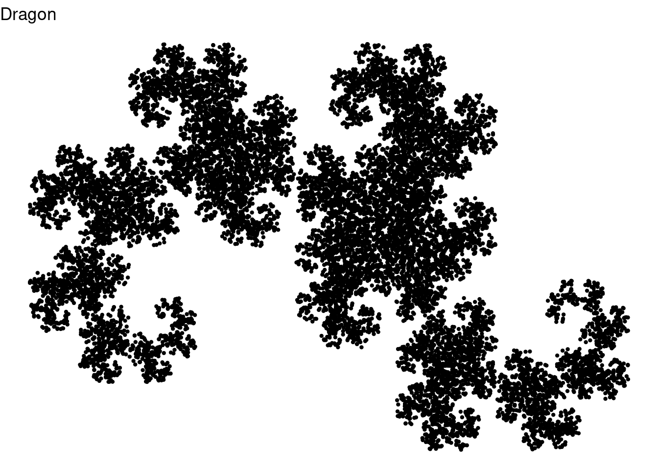
Problem 1b
IFS code for a 5-sided crystal.
# Input a number for n.
# Start with n = 100 until you get the code debugged.
# Then use n = 10000 or 15000 or 20000 or more if needed.
# Use fig.asp = 1 for a square frame.
  n = 10000

# Input the A matrices and the b vectors
  A1 = matrix(c(0.382, 0, 0, 0.382), nrow = 2, byrow = TRUE)
  # A2 = matrix(c(-(1/2), -(1/2), 1/2, -(1/2)), nrow = 2, byrow = TRUE)

  b1 = c(0.3072, 0.6190)
  b2 = c(0.6033, 0.4044)
  b3 = c(0.0139, 0.4044)
  b4 = c(0.1253, 0.0595)
  b5 = c(0.4920, 0.0595)

# Clear and then initialize the data frame with a random vector x
  df <- NULL
  x <- runif(2, 0.0, 1.0)
  df <- data.frame(x = x[1], y = x[2])

# Fractal function.
# Change the cumulative probabilities and add lines as needed.
  Fractal <- function(){
    p = runif(1, 0.0, 1.0) #Computes a random probability p
    if (p <= 1/5) {x <<- A1 %*% x + b1}
    else if (p <= 2/5) {x <<- A1 %*% x + b2}
    else if (p <= 3/5) {x <<- A1 %*% x + b3}
    else if (p <= 4/5) {x <<- A1 %*% x + b4}
    else {x <<- A1 %*% x + b5}
    }

#Loop using the fractal function to fill the data frame with points
  for(i in 1:n) {Fractal()
  df = rbind(df, data.frame(x = x[1], y = x[2]))}

# Scatterplot of the data frame.
# Change title and color as desired.
  ggplot(df, aes(x,y)) + geom_point(color = "black", size = 0.8) +
  ggtitle("5-sided Crystal") + theme_void()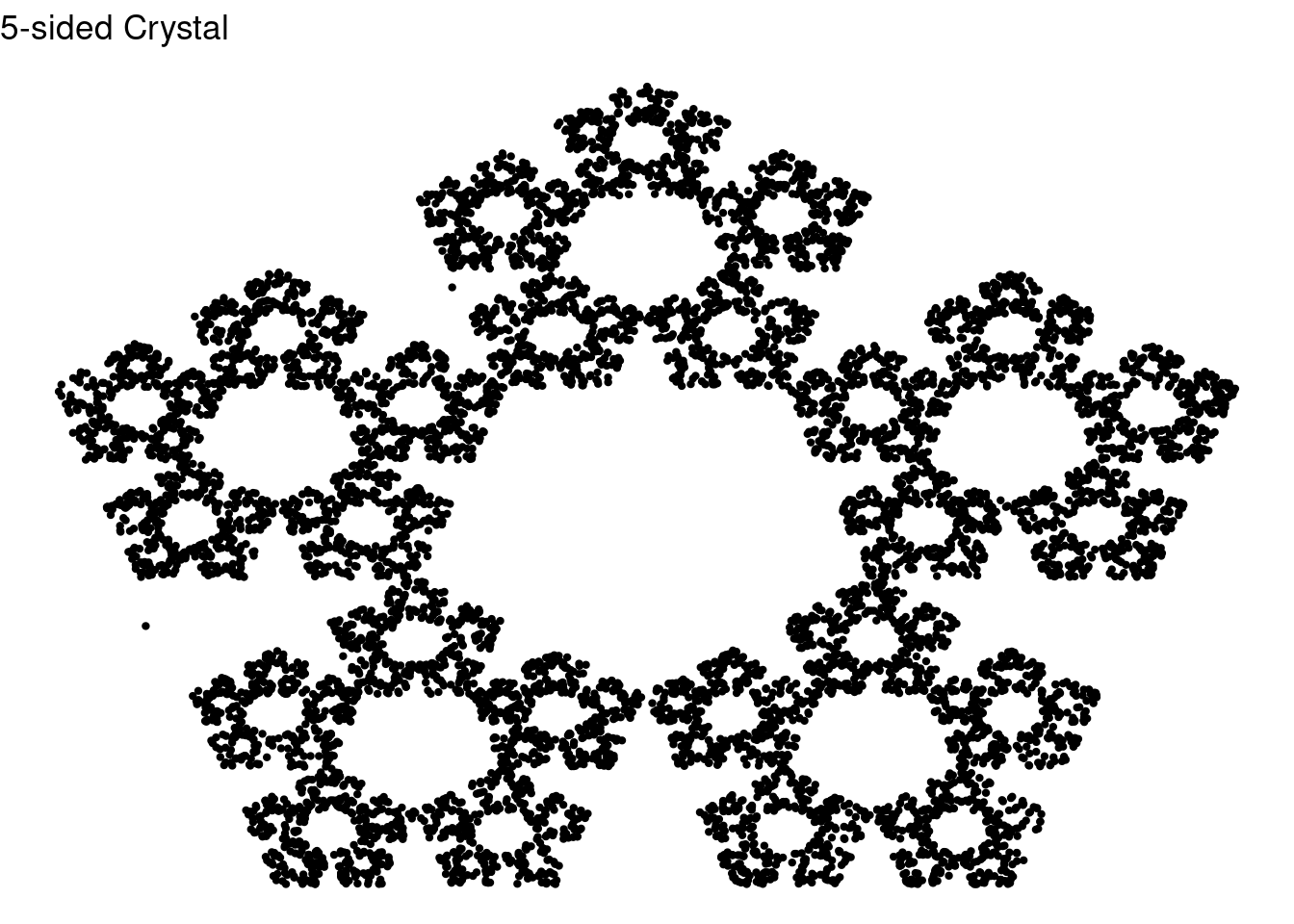
Problem 1c
IFS code for a Sierpinski carpet
# Input a number for n.
# Start with n = 100 until you get the code debugged.
# Then use n = 10000 or 15000 or 20000 or more if needed.
# Use fig.asp = 1 for a square frame.
  n = 10000

# Input the A matrices and the b vectors
  A1 = matrix(c(1/3, 0, 0, 1/3), nrow = 2, byrow = TRUE)
  # A2 = matrix(c(-(1/2), -(1/2), 1/2, -(1/2)), nrow = 2, byrow = TRUE)

  b1 = c(0,0)
  b2 = c(1/3, 0)
  b3 = c(2/3, 0)
  b4 = c(0, 1/3)
  b5 = c(2/3, 1/3)
  b6 = c(0, 2/3)
  b7 = c(1/3, 2/3)
  b8 = c(2/3, 2/3)

# Clear and then initialize the data frame with a random vector x
  df <- NULL
  x <- runif(2, 0.0, 1.0)
  df <- data.frame(x = x[1], y = x[2])

# Fractal function.
# Change the cumulative probabilities and add lines as needed.
  Fractal <- function(){
    p = runif(1, 0.0, 1.0) #Computes a random probability p
    if (p <= 1/8) {x <<- A1 %*% x + b1}
    else if (p <= 2/8) {x <<- A1 %*% x + b2}
    else if (p <= 3/8) {x <<- A1 %*% x + b3}
    else if (p <= 4/8) {x <<- A1 %*% x + b4}
    else if (p <= 5/8) {x <<- A1 %*% x + b5}
    else if (p <= 6/8) {x <<- A1 %*% x + b6}
    else if (p <= 7/8) {x <<- A1 %*% x + b7}
    else {x <<- A1 %*% x + b8}
    }

#Loop using the fractal function to fill the data frame with points
  for(i in 1:n) {Fractal()
  df = rbind(df, data.frame(x = x[1], y = x[2]))}

# Scatterplot of the data frame.
# Change title and color as desired.
  ggplot(df, aes(x,y)) + geom_point(color = "black", size = 0.8) +
  ggtitle("Sierpinkski Carpet") + theme_void()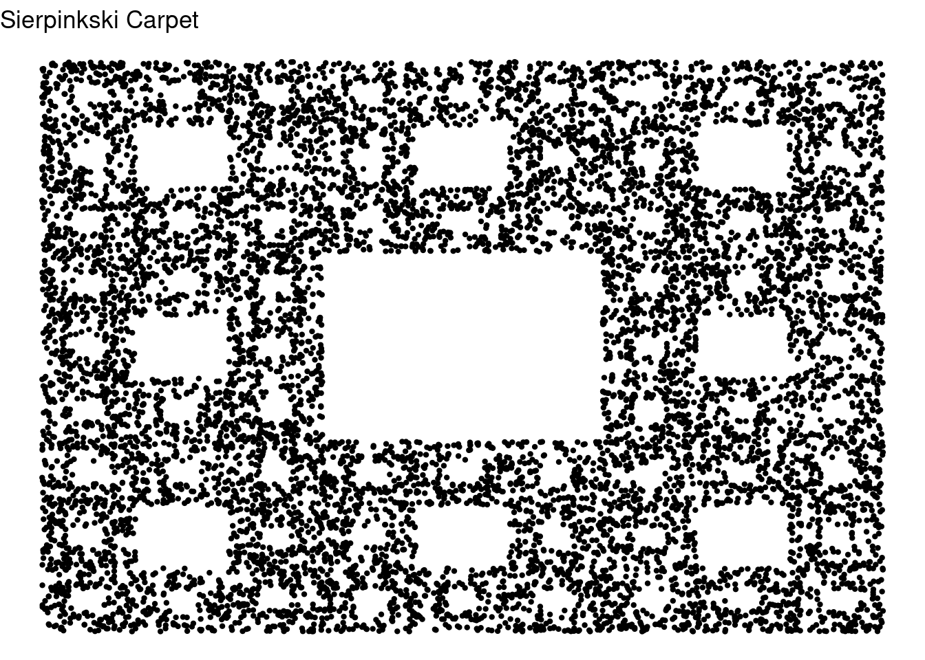
Problem 1d
IFS code for a nautilus
# Input a number for n.
# Start with n = 100 until you get the code debugged.
# Then use n = 10000 or 15000 or 20000 or more if needed.
# Use fig.asp = 1 for a square frame.
  n = 10000

# Input the A matrices and the b vectors
  A1 = matrix(c(0.8607, 0.4015, -0.4023, 0.8619), nrow = 2, byrow = TRUE)
  A2 = matrix(c(0.0950, -0.0010, 0.2370, 0.0020), nrow = 2, byrow = TRUE)
  A3 = matrix(c(0.1509, 0.0, 0.0, 0.1469), nrow = 2, byrow = TRUE)
  A4 = matrix(c(0.3243, -0.0022, 0.0058, 0.0013), nrow = 2, byrow = TRUE)

  b1 = c(0.1085, 0.0751)
  b2 = c(-0.7469, 0.0473)
  b3 = c(-0.5632, 0.0320)
  b4 = c(-0.5579, -0.1397)
  #b5 = c(2/3, 1/3)
  #b6 = c(0, 2/3)
  #b7 = c(1/3, 2/3)
  #b8 = c(2/3, 2/3)

# Clear and then initialize the data frame with a random vector x
  df <- NULL
  x <- runif(2, 0.0, 1.0)
  df <- data.frame(x = x[1], y = x[2])

# Fractal function.
# Change the cumulative probabilities and add lines as needed.
  Fractal <- function(){
    p = runif(1, 0.0, 1.0) #Computes a random probability p
    if (p <= 0.93) {x <<- A1 %*% x + b1}
    else if (p <= 0.02) {x <<- A2 %*% x + b2}
    else if (p <= 0.03) {x <<- A3 %*% x + b3}
    else if (p <= 0.02) {x <<- A4 %*% x + b4}
    #else if (p <= 5/8) {x <<- A1 %*% x + b5}
    #else if (p <= 6/8) {x <<- A1 %*% x + b6}
    #else if (p <= 7/8) {x <<- A1 %*% x + b7}
    #else {x <<- A1 %*% x + b8}
    }

#Loop using the fractal function to fill the data frame with points
  for(i in 1:n) {Fractal()
  df = rbind(df, data.frame(x = x[1], y = x[2]))}

# Scatterplot of the data frame.
# Change title and color as desired.
  ggplot(df, aes(x,y)) + geom_point(color = "black", size = 0.8) +
  ggtitle("Nautilus") + theme_void()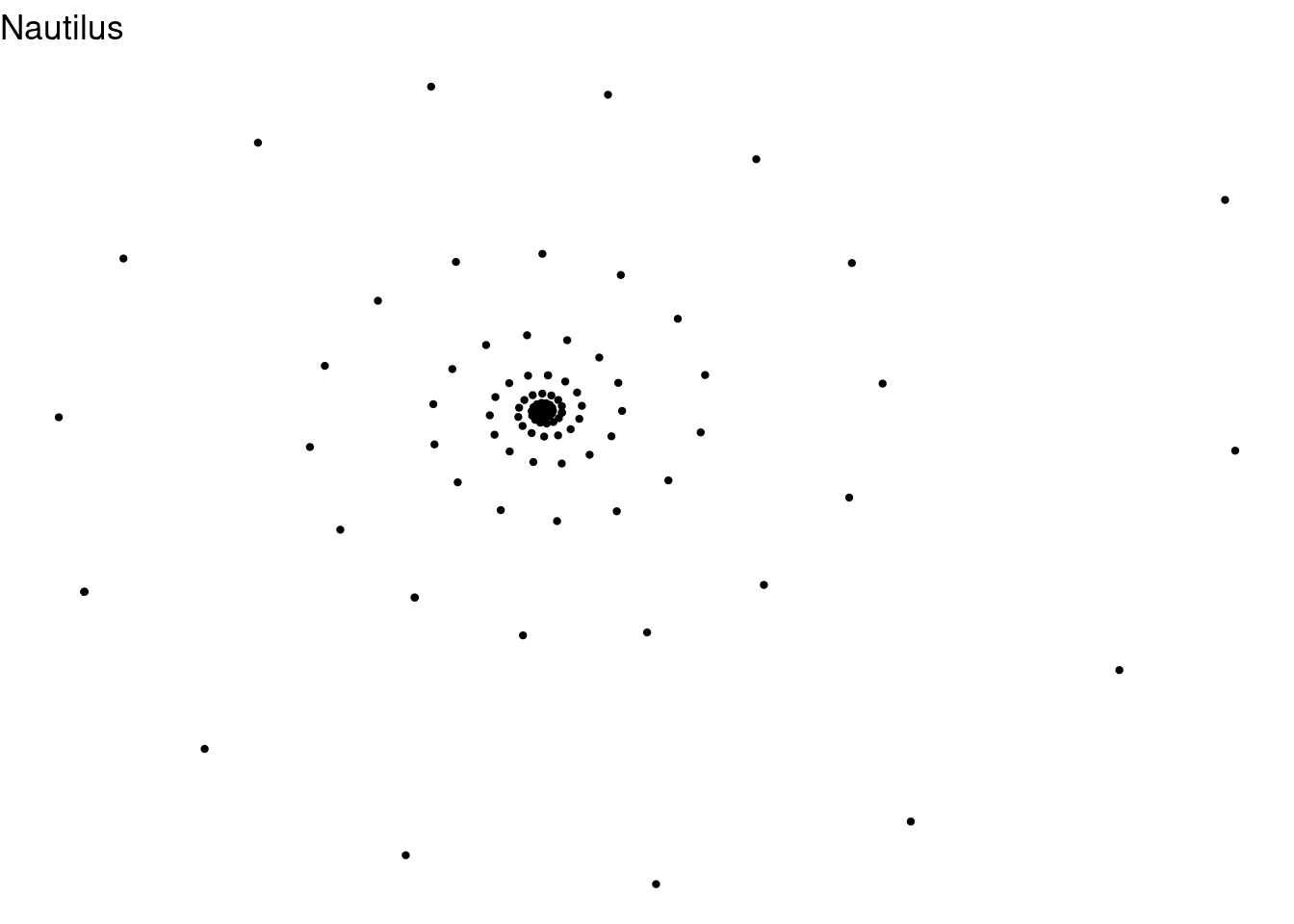
Problem 1e
IFS code for Tree A:
# Input a number for n.
# Start with n = 100 until you get the code debugged.
# Then use n = 10000 or 15000 or 20000 or more if needed.
# Use fig.asp = 1 for a square frame.
  n = 10000

# Input the A matrices and the b vectors
  A1 = matrix(c(0, 0, 0, 0.5), nrow = 2, byrow = TRUE)
  A2 = matrix(c(0.42, -0.42, 0.42, 0.42), nrow = 2, byrow = TRUE)
  A3 = matrix(c(0.42, 0.42, -0.42, 0.42), nrow = 2, byrow = TRUE)
  A4 = matrix(c(0.1, 0, 0, 0.1), nrow = 2, byrow = TRUE)

  b1 = c(0,0)
  b2 = c(0,0.2)
  #b3 = c(-0.5632, 0.0320)
  #b4 = c(-0.5579, -0.1397)
  #b5 = c(2/3, 1/3)
  #b6 = c(0, 2/3)
  #b7 = c(1/3, 2/3)
  #b8 = c(2/3, 2/3)

# Clear and then initialize the data frame with a random vector x
  df <- NULL
  x <- runif(2, 0.0, 1.0)
  df <- data.frame(x = x[1], y = x[2])

# Fractal function.
# Change the cumulative probabilities and add lines as needed.
  Fractal <- function(){
    p = runif(1, 0.0, 1.0) #Computes a random probability p
    if (p <= 0.05) {x <<- A1 %*% x + b1}
    else if (p <= 0.15) {x <<- A4 %*% x + b2}
    else if (p <= 0.40) {x <<- A3 %*% x + b2}
    else if (p <= 0.40) {x <<- A %*% x + b2}
    #else if (p <= 5/8) {x <<- A1 %*% x + b5}
    #else if (p <= 6/8) {x <<- A1 %*% x + b6}
    #else if (p <= 7/8) {x <<- A1 %*% x + b7}
    #else {x <<- A1 %*% x + b8}
    }

#Loop using the fractal function to fill the data frame with points
  for(i in 1:n) {Fractal()
  df = rbind(df, data.frame(x = x[1], y = x[2]))}

# Scatterplot of the data frame.
# Change title and color as desired.
  ggplot(df, aes(x,y)) + geom_point(color = "black", size = 0.8) +
  ggtitle("Tree A") + theme_void()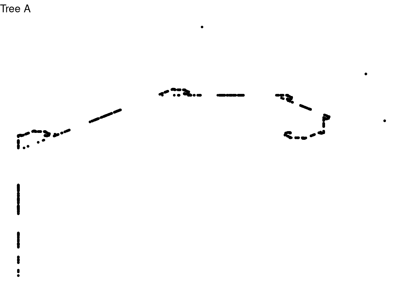
Problem 1f
IFS code for Tree B:
# Input a number for n.
# Start with n = 100 until you get the code debugged.
# Then use n = 10000 or 15000 or 20000 or more if needed.
# Use fig.asp = 1 for a square frame.
  n = 10000

# Input the A matrices and the b vectors
  A1 = matrix(c(0.195, 0.344, 0.443, 0.4431), nrow = 2, byrow = TRUE)
  A2 = matrix(c(0.462, 0.414, -0.252, 0.361), nrow = 2, byrow = TRUE)
  A3 = matrix(c(-0.058, -0.070, 0.453, -0.111), nrow = 2, byrow = TRUE)
  A4 = matrix(c(-0.035, 0.070, -0.469, -0.022), nrow = 2, byrow = TRUE)
  A5 = matrix(c(-0.637, 0, 0, 0.501), nrow = 2, byrow = TRUE)

  b1 = c(0.4431,0.2452)
  b2 = c(0.2511,0.5692)
  b3 = c(0.5976, 0.0969)
  b4 = c(0.4884, 0.5069)
  b5 = c(0.8562, 0.2513)
  #b6 = c(0, 2/3)
  #b7 = c(1/3, 2/3)
  #b8 = c(2/3, 2/3)

# Clear and then initialize the data frame with a random vector x
  df <- NULL
  x <- runif(2, 0.0, 1.0)
  df <- data.frame(x = x[1], y = x[2])

# Fractal function.
# Change the cumulative probabilities and add lines as needed.
  Fractal <- function(){
    p = runif(1, 0.0, 1.0) #Computes a random probability p
    if (p <= 0.1699) {x <<- A1 %*% x + b1}
    else if (p <= 0.1811) {x <<- A2 %*% x + b2}
    else if (p <= 0.2161) {x <<- A3 %*% x + b3}
    else if (p <= 0.2198) {x <<- A4 %*% x + b4}
    else if (p <= 0.2131) {x <<- A5 %*% x + b5}
    #else if (p <= 6/8) {x <<- A1 %*% x + b6}
    #else if (p <= 7/8) {x <<- A1 %*% x + b7}
    #else {x <<- A1 %*% x + b8}
    }

#Loop using the fractal function to fill the data frame with points
  for(i in 1:n) {Fractal()
  df = rbind(df, data.frame(x = x[1], y = x[2]))}

# Scatterplot of the data frame.
# Change title and color as desired.
  ggplot(df, aes(x,y)) + geom_point(color = "black", size = 0.8) +
  ggtitle("Tree A") + theme_void()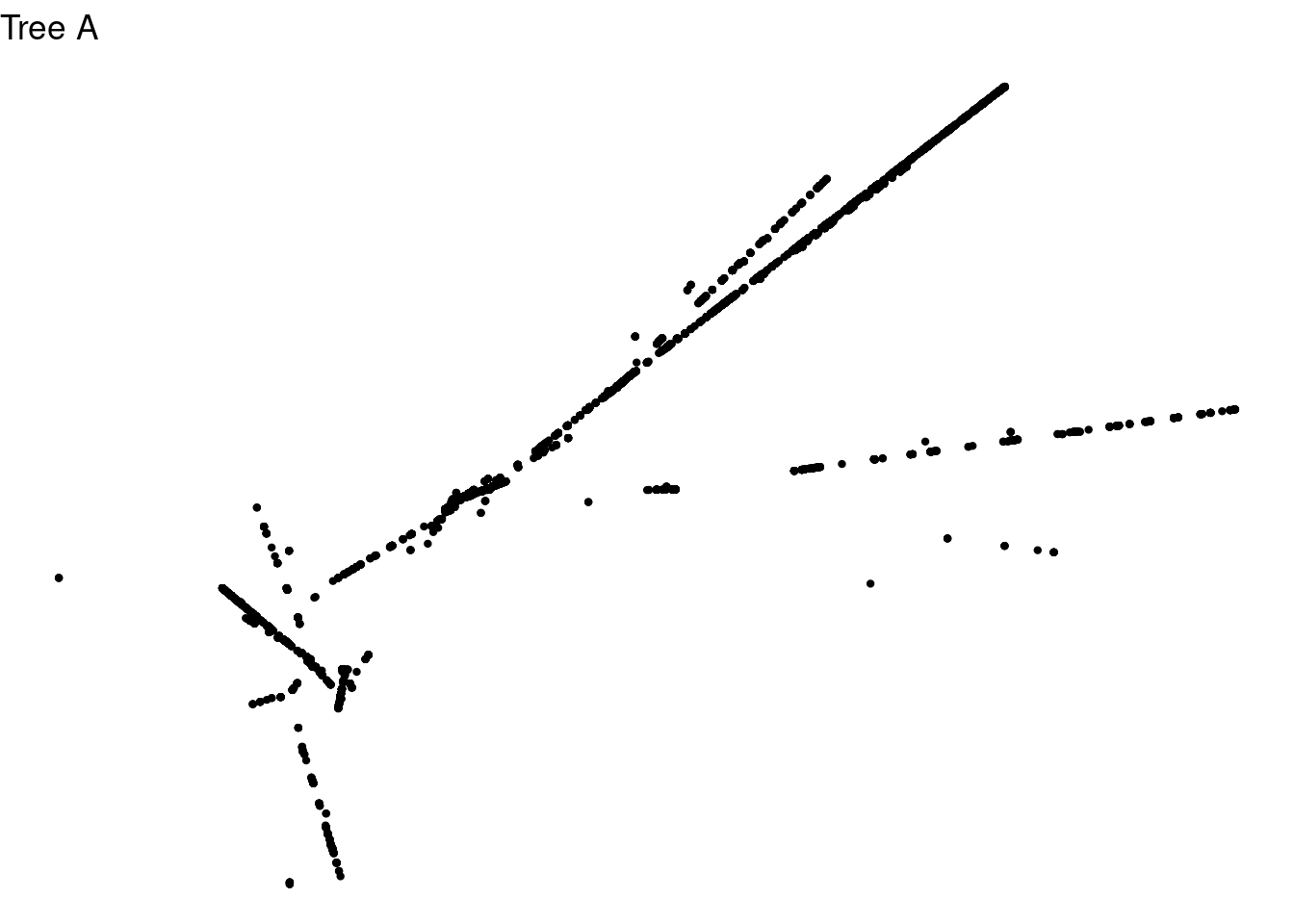
Problem 1f
IFS code for Tree C:
# Input a number for n.
# Start with n = 100 until you get the code debugged.
# Then use n = 10000 or 15000 or 20000 or more if needed.
# Use fig.asp = 1 for a square frame.
  n = 100

# Input the A matrices and the b vectors
  A1 = matrix(c(0.195, 0.344, 0.443, 0.4431), nrow = 2, byrow = TRUE)
  A2 = matrix(c(0.462, 0.414, -0.252, 0.361), nrow = 2, byrow = TRUE)
  A3 = matrix(c(-0.058, -0.070, 0.453, -0.111), nrow = 2, byrow = TRUE)
  A4 = matrix(c(-0.035, 0.070, -0.469, -0.022), nrow = 2, byrow = TRUE)
  A5 = matrix(c(-0.637, 0, 0, 0.501), nrow = 2, byrow = TRUE)

  b1 = c(0.4431,0.2452)
  b2 = c(0.2511,0.5692)
  b3 = c(0.5976, 0.0969)
  b4 = c(0.4884, 0.5069)
  b5 = c(0.8562, 0.2513)
  #b6 = c(0, 2/3)
  #b7 = c(1/3, 2/3)
  #b8 = c(2/3, 2/3)

# Clear and then initialize the data frame with a random vector x
  df <- NULL
  x <- runif(2, 0.0, 1.0)
  df <- data.frame(x = x[1], y = x[2])

# Fractal function.
# Change the cumulative probabilities and add lines as needed.
  Fractal <- function(){
    p = runif(1, 0.0, 1.0) #Computes a random probability p
    if (p <= 0.1699) {x <<- A1 %*% x + b1}
    else if (p <= 0.1811) {x <<- A2 %*% x + b2}
    else if (p <= 0.2161) {x <<- A3 %*% x + b3}
    else if (p <= 0.2198) {x <<- A4 %*% x + b4}
    else if (p <= 0.2131) {x <<- A5 %*% x + b5}
    #else if (p <= 6/8) {x <<- A1 %*% x + b6}
    #else if (p <= 7/8) {x <<- A1 %*% x + b7}
    #else {x <<- A1 %*% x + b8}
    }

#Loop using the fractal function to fill the data frame with points
  for(i in 1:n) {Fractal()
  df = rbind(df, data.frame(x = x[1], y = x[2]))}

# Scatterplot of the data frame.
# Change title and color as desired.
  ggplot(df, aes(x,y)) + geom_point(color = "black", size = 0.8) +
  ggtitle("Tree A") + theme_void()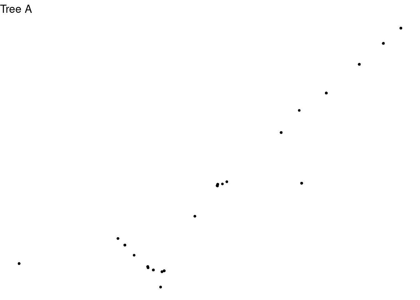
Problem 2
Use Newton’s method to find all roots on the given interval. Round to 3 decimal places as needed. Graph the function.
Problem 2a
# Input the functions f and fprime
  f <- function(x) {(2*x)^3 + (11*x)^2 - (7*x) - 6}
  fprime <- function(x) {(6*x)^2 + (22*x) - 7}

# Graph f to see how many roots there are; Adjust xlim as needed
  x <- -7:2
  ggplot(data.frame(x), aes(x)) +
  stat_function(fun = f, color = "blue", size = 1) + xlim(-7, 2) +
  geom_hline(yintercept = 0) + geom_vline(xintercept = 0) +
    ggtitle("problem 2a")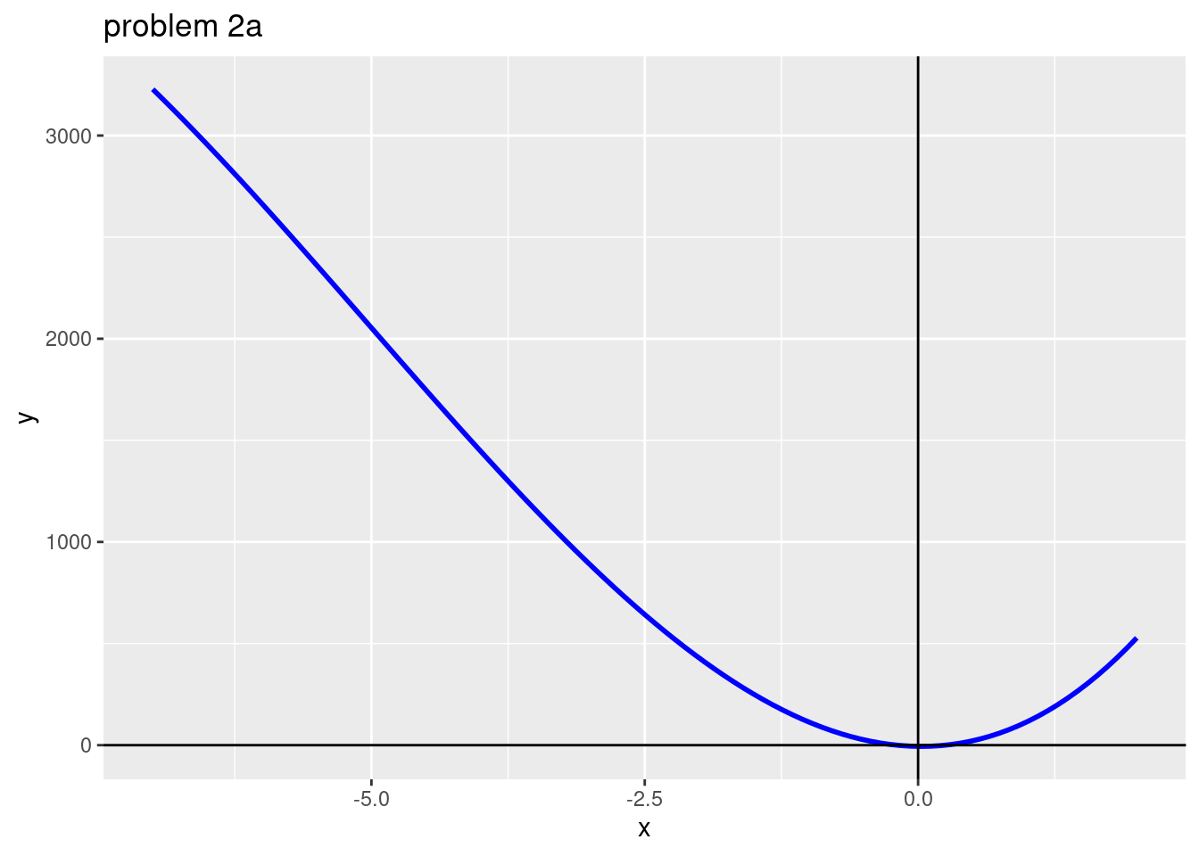
# Newton’s method function
  Newton <- function(f, fprime, x0) {
  tol = 0.0001
  maxiter = 100
  icount = 1
  x = x0
  while(abs(f(x)) > tol & icount < maxiter)
    {x = x - f(x)/fprime(x) # This is the Newton’s method formula
    icount = icount + 1}
  print(round(x,4))}
# Call the function to find each root; Provide an appropriate value for the initial guess x0
  Newton(f, fprime, 0)
## [1] -15.1794Problem 2b
# Input the functions f and fprime
  f <- function(x) {(3*x)^3 - (x)^2 - (15*x) + 5}
  fprime <- function(x) {(9*x)^2 - (2*x) - 15}

# Graph f to see how many roots there are; Adjust xlim as needed
  x <- -3:3
  ggplot(data.frame(x), aes(x)) +
  stat_function(fun = f, color = "blue", size = 1) + xlim(-3, 3) +
  geom_hline(yintercept = 0) + geom_vline(xintercept = 0) +
    ggtitle("problem 2b")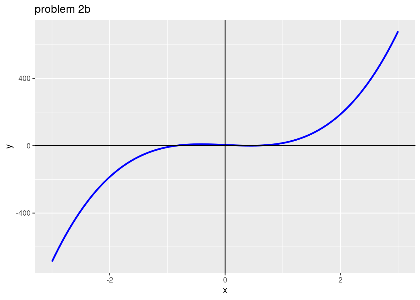
# Newton’s method function
  Newton <- function(f, fprime, x0) {
  tol = 0.0001
  maxiter = 100
  icount = 1
  x = x0
  while(abs(f(x)) > tol & icount < maxiter)
    {x = x - f(x)/fprime(x) # This is the Newton’s method formula
    icount = icount + 1}
  print(round(x,4))}
# Call the function to find each root; Provide an appropriate value for the initial guess x0
  Newton(f, fprime, 0)
## [1] -0.8597Problem 2c
# Input the functions f and fprime
  f <- function(x) {(1.7*x) * sin(5.2 * x) + 1}
  fprime <- function(x) {1.7 * sin(5.2*x) + (8.84*x) * cos(5.2 * x)}

# Graph f to see how many roots there are; Adjust xlim as needed
  x <- 0:2
  ggplot(data.frame(x), aes(x)) +
  stat_function(fun = f, color = "blue", size = 1) + xlim(0, 2) +
  geom_hline(yintercept = 0) + geom_vline(xintercept = 0) +
    ggtitle("problem 2c")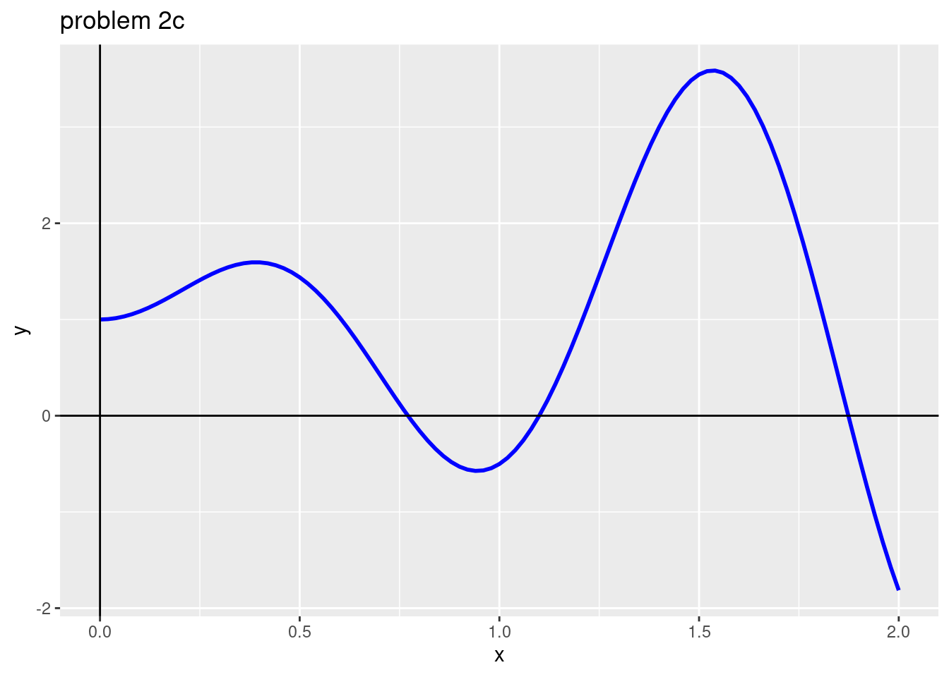
# Newton’s method function
  Newton <- function(f, fprime, x0) {
  tol = 0.0001
  maxiter = 100
  icount = 1
  x = x0
  while(abs(f(x)) > tol & icount < maxiter)
    {x = x - f(x)/fprime(x) # This is the Newton’s method formula
    icount = icount + 1}
  print(round(x,4))}

# Call the function to find each root; Provide an appropriate value for the initial guess x0
  Newton(f, fprime, 1)
## [1] 1.0998Problem 3.
Use Newton’s method to find all points of intersection of the given functions. Round to 4 decimal places as needed. Graph the two functions on the same set of axes.
  # Define f and g

  f <- function(x) {x + 2}
  g <- function(x) {exp(1)^(2*x)}
  x <- -3:10

  # Plot the two graphs.

  ggplot(data.frame(x), aes(x)) +
    stat_function(fun = f, color = "red", size = 1) +
    stat_function(fun = g, color = "blue", size = 1) +
    xlim(-3, 1.5) +
    ylim(-1, 10) + # This adjustment is necessary to actually be able to see "f(x)". It gives a warning but that's a necessary evil I think.
    geom_hline(yintercept = 0) +
    geom_vline(xintercept = 0)
## Warning: Removed 8 row(s) containing missing values (geom_path).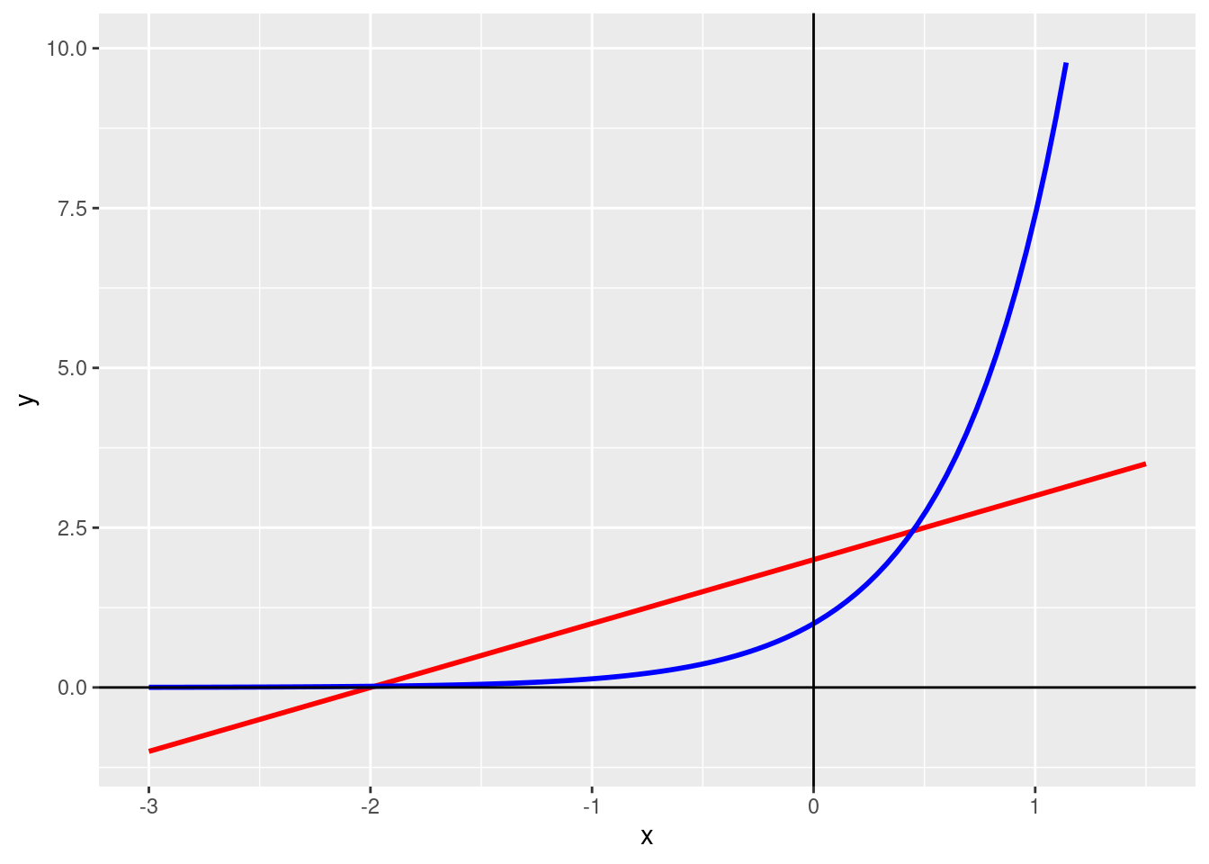
# Input the functions h and hprime
  h <- function(x) {(x+2) - exp(1)^(2*x)}
  hprime <- function(x) {1 - (2 * exp(1)^(2 * x))}

# Newton’s method function
  Newton <- function(h, hprime, x0) {
  tol = 0.0001
  maxiter = 100
  icount = 1
  x = x0
  while(abs(h(x)) > tol & icount < maxiter)
    {x = x - h(x)/hprime(x) # This is the Newton’s method formula
    icount = icount + 1}
  print(round(x, digits = 4))}

# Call the function to find each root; Provide an appropriate value for the initial guess x0
  Newton(h, hprime, 0)
## [1] 0.4476I’m not entirely sure how to make this problem find both intersections. The one in output IS correct, but there should be two intersections I believe, not one. Regardless, this seems mostly correct.
Problem 3b
  # Define f and g

  f <- function(x) {exp(1)^x + log(x)}
  g <- function(x) {4}
  x <- -1:3

  # Plot the two graphs.

  ggplot(data.frame(x), aes(x)) +
    stat_function(fun = f, color = "red", size = 1) +
    stat_function(fun = g, color = "blue", size = 1) +
    xlim(-1, 2) +
    ylim(-1, 5) +
    geom_hline(yintercept = 0) +
    geom_vline(xintercept = 0)
## Warning in log(x): NaNs produced## Warning: Removed 54 row(s) containing missing values (geom_path).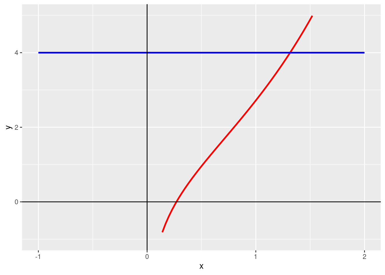
# Input the functions h and hprime
  h <- function(x) {(exp(1)^x + log(x)) - 4}
  hprime <- function(x) {exp(1)^x - (1/x)}

# Newton’s method function
  Newton <- function(h, hprime, x0) {
  tol = 0.0001
  maxiter = 100
  icount = 1
  x = x0
  while(abs(h(x)) > tol & icount < maxiter)
    {x = x - h(x)/hprime(x) # This is the Newton’s method formula
    icount = icount + 1}
  print(round(x, digits = 4))}

# Call the function to find each root; Provide an appropriate value for the initial guess x0
  Newton(h, hprime, 1)
## [1] 1.3153Problem 4.
Problem 4a
Draw at least two graphs of the entire Mandelbrot set with different color schemes.
mb <- mandelbrot(iterations = 500)
  cols <- mandelbrot_palette(brewer.pal(11, "RdYlBu"), fold = FALSE)
  plot(mb, col = cols, transform = "log")
mb <- mandelbrot(iterations = 500)
  cols <- mandelbrot_palette(brewer.pal(12, "Set3"), fold = FALSE)
  plot(mb, col = cols, transform = "log")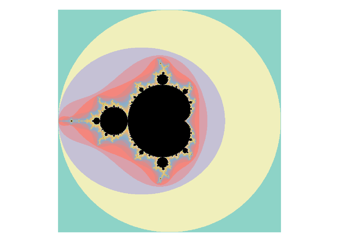
Problem 4b
Use xlim = c(-0.75, 0.72), ylim = c(0.17, 0.2) to zoom in on Seahorse Valley.
mb <- mandelbrot(xlim = c(-0.75, -0.72), ylim = c(0.17, 0.2), iterations = 500)
  cols <- mandelbrot_palette(brewer.pal(11, "RdYlBu"), fold = FALSE)
  plot(mb, col = cols, transform = "log")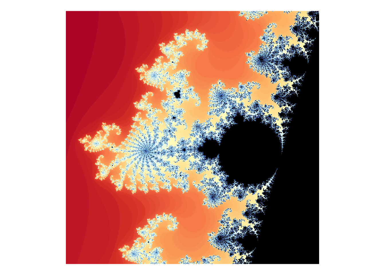
Problem 4c
mb <- mandelbrot(xlim = c(-0.9, -0.7), ylim = c(0, 0.4), iterations = 500)
  cols <- mandelbrot_palette(brewer.pal(11, "RdYlBu"), fold = FALSE)
  plot(mb, col = cols, transform = "log")
Problem 4d
Zoom in on Elephant Valley
mb <- mandelbrot(xlim = c(0.271, 0.276), ylim = c(-0.008, -0.004), iterations = 500)
  cols <- mandelbrot_palette(brewer.pal(11, "RdYlBu"), fold = FALSE)
  plot(mb, col = cols, transform = "log")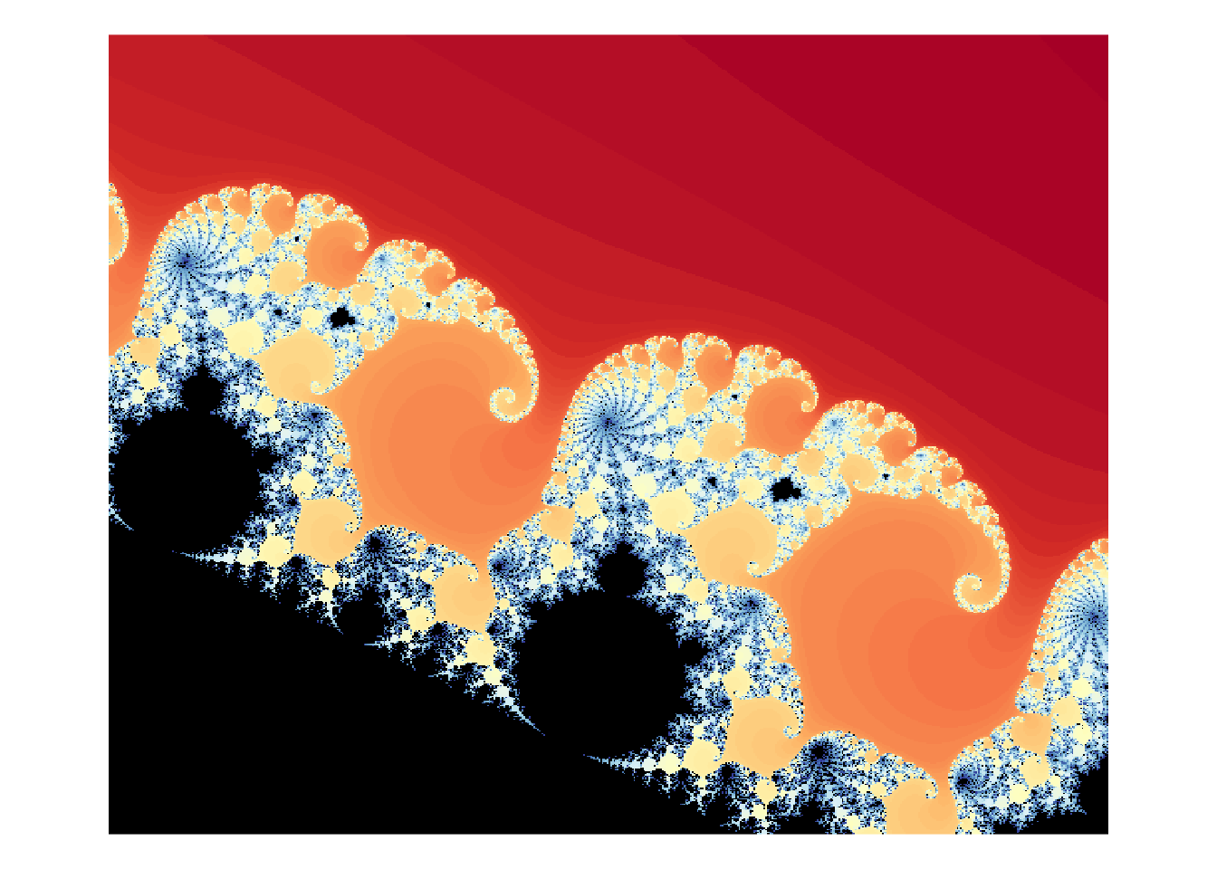
Problem 4e
mb <- mandelbrot(xlim = c(0.248, 0.28), ylim = c(-0.01, 0.01), iterations = 500)
  cols <- mandelbrot_palette(brewer.pal(11, "RdYlBu"), fold = FALSE)
  plot(mb, col = cols, transform = "log")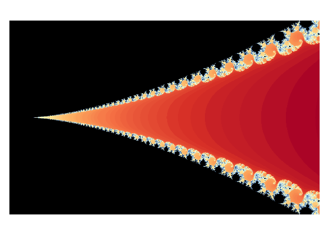
Problem 4f
Zoom in on at least one other region on the boundary of the Mandelbrot set
mb <- mandelbrot(xlim = c(-0.73405, -0.73395), ylim = c(0.2039, 0.2040), iterations = 1000)
  cols <- mandelbrot_palette(brewer.pal(11, "RdYlBu"), fold = FALSE)
  plot(mb, col = cols, transform = "log")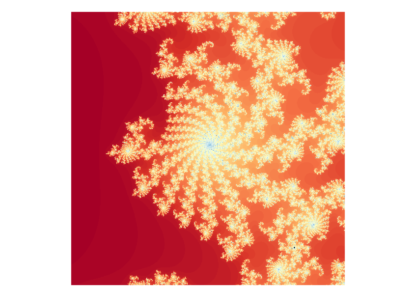
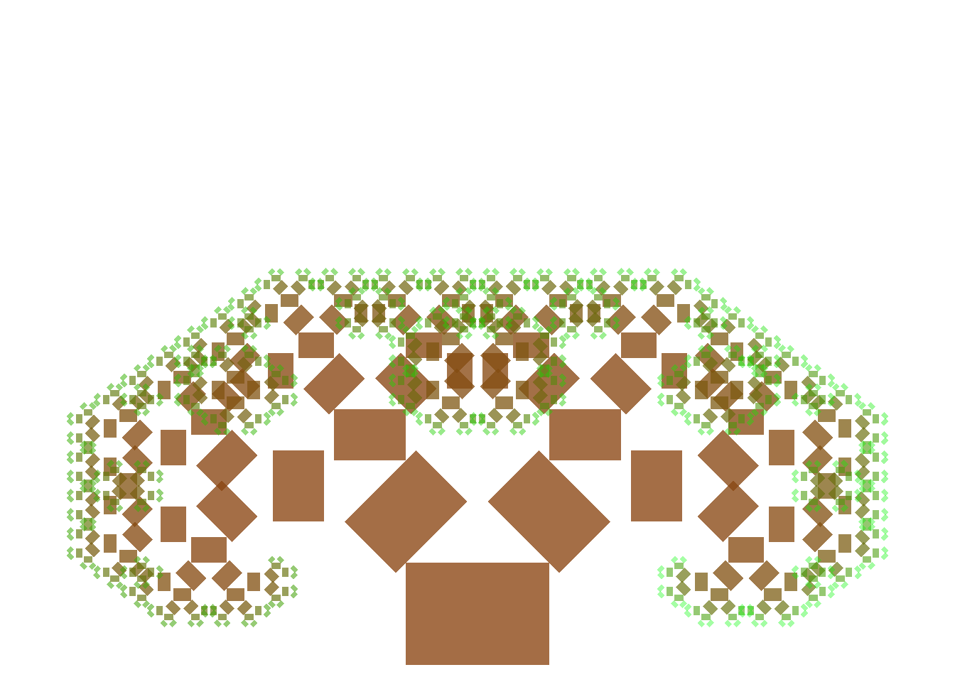
Problem 5 [Pythagorean Tree]
Load the package grid. Run the following code.
grid.newpage()
l = 0.15 # Length of the square
gr <- rectGrob(width=l, height=l, name="gr") # Basic Square
pts <- data.frame(level=1, x=0.5, y=0.1, alfa=0) # Centers of the squares

for (i in 2:10) #10=Deep of the fractal. Feel free to change this
    {df<-pts[pts$level==i-1,] # This == (2 equal signs)
    for (j in 1:nrow(df))
    {pts <- rbind(pts, c(i, df[j,]
    $x-2*l*((1/sqrt(2))^(i-1))*sin(df[j,]$alfa+pi/4)-
    0.5*l*((1/sqrt(2))^(i-2))*sin(df[j,]$alfa+pi/4-3*pi/4),
    df[j,]$y+2*l*((1/sqrt(2))^(i-1))*cos(df[j,]$alfa+pi/4)+
    0.5*l*((1/sqrt(2))^(i-2))*cos(df[j,]$alfa+pi/4-3*pi/4),
    df[j,]$alfa+pi/4))
    pts <- rbind(pts, c(i, df[j,]
    $x-2*l*((1/sqrt(2))^(i-1))*sin(df[j,]$alfa-pi/4)-
    0.5*l*((1/sqrt(2))^(i-2))*sin(df[j,]$alfa-pi/4+3*pi/4),
    df[j,]$y+2*l*((1/sqrt(2))^(i-1))*cos(df[j,]$alfa-pi/4)+
    0.5*l*((1/sqrt(2))^(i-2))*cos(df[j,]$alfa-pi/4+3*pi/4),
    df[j,]$alfa-pi/4))}}

for (i in 1:nrow(pts))
    {grid.draw(editGrob(gr, vp=viewport(x=pts[i,]$x, y=pts[i,]$y,
    w=((1/sqrt(2))^(pts[i,]$level-1)),
    h=((1/sqrt(2))^(pts[i,]$level-1)),
    angle=pts[i,]$alfa*180/pi),
    gp=gpar(col=0, lty="solid",
    fill=rgb(139*(nrow(pts)-i)/(nrow(pts)-1),
    (186*i+69*nrow(pts)-255)/(nrow(pts)-1),
    19*(nrow(pts)-i)/(nrow(pts)-1),
    alpha= (-110*i+200*nrow(pts)-90)/(nrow(pts)-1), max=255))))}