MTH-2520 Homework 4: Vectors Part II

Pr. 1

data <- c(1.2,-3.5,4.3,8.6,-5.1)
summary(data)

   Min. 1st Qu.  Median    Mean 3rd Qu.    Max. 
   -5.1    -3.5     1.2     1.1     4.3     8.6

cat("The sample mean is",mean(data),"\n")

The sample mean is 1.1

cat("The sample standard deviation is",sd(data),"\n")

The sample standard deviation is 5.614713

cat("The interquartile range is",IQR(data),"\n")

The interquartile range is 7.8

The mean of the data set is 1.1.

The median of the data set is 1.2.

The sample standard deviation is 5.6147128.

The interquartile range is 7.8

Pr. 2

data2 <- c(4.1, 4.3, 4.7, 3.4, 3.9, 5.6, 4.6, NA, 6.6, 5.1, 4.3, 49, NA, 4.4, 6.1)

# I really like this method of formatting. It looks so clean! 

cat("The sample mean is", mean(data2, na.rm = TRUE), "\n")

The sample mean is 8.161538

cat("The standard deviation of this sample is", sd(data2, na.rm = TRUE), "\n")

The standard deviation of this sample is 12.30302

cat("The median of this sample is", median(data2, na.rm = TRUE), "\n")

The median of this sample is 4.6

cat("The interquartile range of this sample is", IQR(data2, na.rm = TRUE), "\n")

The interquartile range of this sample is 1.3

Pr. 3

xdata <- read.csv("hw4_x.csv",sep="")
cat("The type of data is", typeof(xdata), "\n")

The type of data is list

summary(xdata)

       x        
 Min.   : 13.0  
 1st Qu.:238.8  
 Median :526.0  
 Mean   :488.0  
 3rd Qu.:751.8  
 Max.   :991.0

cat("The standard deviation of ydata is", sd(xdata$x, na.rm = TRUE), "\n")

The standard deviation of ydata is 298.2539

cat("The interquartile rnage of ydata is", IQR(xdata$x, na.rm = TRUE), "\n")

The interquartile rnage of ydata is 513

hist(xdata$x,main="Histogram of the Data Set x",xlab="x",col="magenta")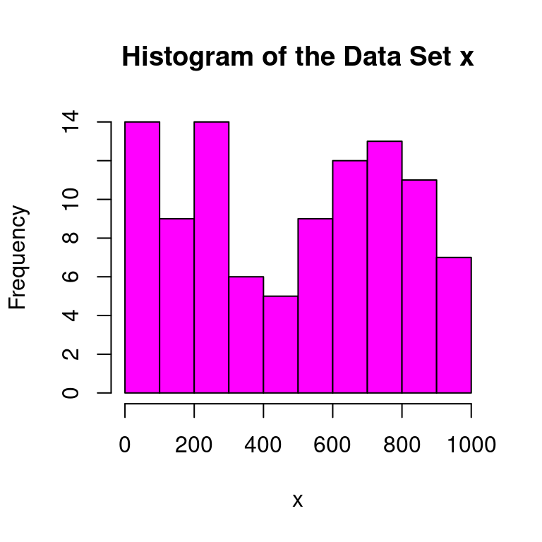

Pr. 4

ydata <- read.csv("hw4_y.csv",sep="")
cat("The type of data is", typeof(ydata), "\n")

The type of data is list

summary(ydata)

       y        
 Min.   : 36.0  
 1st Qu.:271.5  
 Median :543.0  
 Mean   :528.3  
 3rd Qu.:801.5  
 Max.   :997.0

cat("The standard deviation of ydata is", sd(ydata$y), "\n")

The standard deviation of ydata is 296.5066

cat("The interquartile rnage of ydata is", IQR(ydata$y), "\n")

The interquartile rnage of ydata is 530

hist(ydata$y,main="Histogram of the Data Set y", xlab="y",col="yellow")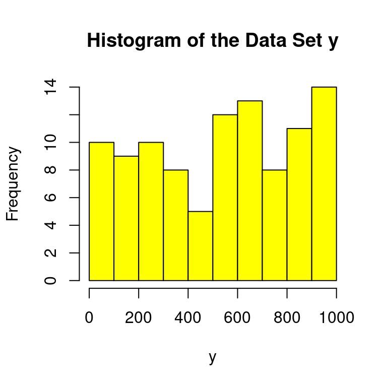

Pr. 5

Pr. 5a

# Problem 5a. 

x <- c(1, 2, 5, 9, 11)
y <- c(2, 5, 1, 0, 23)

intersect(x, y)

[1] 1 2 5

Pr. 5b

# Problem 5b. 
union(x, y)

[1]  1  2  5  9 11  0 23

c(x, y)

 [1]  1  2  5  9 11  2  5  1  0 23

# The difference is that while c(x, y) includes all of the data from both vectors, union removes the duplicates. So, there's only one instance of "2" inside of the union made vector for instance.

Pr. 5c and 5d

# Problem 5c and 5d 
cat("The set difference of x and y is", setdiff(x, y), "\n"); cat("The set difference of y and x is", setdiff(y, x), "\n")

The set difference of x and y is 9 11

The set difference of y and x is 0 23

Pr. 5e

# Problem 5e.
# Symmetric difference in my understanding can be described as the union of the two above set difference calculations. So if I was to do this by hand it would look like c(9, 11, 0, 23).

diff_X_Y <- setdiff(x, y); diff_Y_X <- setdiff(y, x) 

cat("The symmetric difference is", union(diff_X_Y, diff_Y_X), "\n")

The symmetric difference is 9 11 0 23

Pr. 6

6a

# Pr. 6a: Adding the vectors
cat("x plus y is", x + y, "\n")

x plus y is 3 7 6 9 34

6b

# Pr. 6b: Subtracting the vectors
cat("4x minus 5y is", (4*x) - (5*y), "\n")

4x minus 5y is -6 -17 15 36 -71

6c

# Pr. 6c: Multiplying the vectors
cat("x multiplied by y is ", x * y, "\n")

x multiplied by y is  2 10 5 0 253

6d

# Pr. 6d: Dividing the vectors
cat("x divided by y is", x / y, "\n")

x divided by y is 0.5 0.4 5 Inf 0.4782609

6e

# Pr. 6e: Dot product of vectors
cat("The dot product of x and y is", dot(x,y), "\n")

The dot product of x and y is 270

6f

# Pr. 6f: Magnitude of x
cat("The magnitude of x is", sqrt(dot(x, x)), "\n")

The magnitude of x is 15.23155

6g

# Pr. 6g: Cumulative sum of x
cat("The cumulative sum of x is", cumsum(x), "\n")

The cumulative sum of x is 1 3 8 17 28

6h

# Pr. 6h: Cumulative product of x
cat("The cumulative product of x is", cumprod(x), "\n")

The cumulative product of x is 1 2 10 90 990

Pr. 7

7a

# Pr. 7a
xint <- unlist(xdata); yint <- unlist(ydata)

7b

# Pr. 7b: Intersection of xint and yint
intersect(xint, yint)

 [1] 253 743 849 166 920 373 131 941 102 297 874  75 837  74 606

7c

# Pr. 7c: Set difference of xint and yint
setdiff(xint, yint)

 [1] 440 787 270 680 757 199 331 725 261 774  43  66  64 189 641 872  13 790 319
[20] 947 303 493  95 543 579 896 296 125 563  89 568 479 217 327 281 282 667 646
[39] 438 509 687 323 569  63 706 814 191 862 991 246 877 926 263 792 909 723 895
[58] 664 126  97 661 256 924 406 576 783 643 852 501 750 277 285  51 636 793 213
[77]  60 718  23 879 642 117

7d

# Pr. 7d: Set difference of yint and xint
setdiff(yint, xint)

 [1] 921 164 310 993 239 258 551 397 113 703  41 923 809  85 502 435 586 657 504
[20] 291 966 954 276 658  45 811 939 592 659 678 538 742 540 517 707 441 859 639
[39] 997 772 873 103 519  44 518 815 912 326 453 387 128  50 656 755 204 631 378
[58] 756 534 195 890 882 918 364 799 306 620 637 300 974 546 832 467  36 221 248
[77] 160 660  68 610

7e

# Pr. 7e: Finding specific integers in xint or yint.
problem_7e <- c(42, 373, 678)
problem_7e %in% xint

[1] FALSE  TRUE FALSE

problem_7e %in% yint

[1] FALSE  TRUE  TRUE

The results show that c(42, 373, 678) is nowhere to be found in xint. 373 and 678 are found in yint though.

Pr. 8

8a

# Pr. 8a
i_a <- 1:200
sum(i_a^2)

[1] 2686700

n <- 200
n * (n + 1) * ((2 * n) + 1) / 6

[1] 2686700

8b

# Pr. 8b
i_b <- 10:100
sum(i_b^3 + (4 * i_b^2))

[1] 26852735

8c

# Pr. 8c
i_c <- 1:15
sum((2^{i_c} / i_c) + (3^{i_c} / i_c^2))

[1] 108538

8d

# Pr. 8d
i_d <- 0:15
sum(2^{i_d} / factorial(i_d))

[1] 7.389056

# To check that this actually converges with e^2 we can just do this.
cat("This is eulers number squared", exp(2), "\n")

This is eulers number squared 7.389056

8e

# Pr. 8e
i_e <- 1:10^6
4 * sum(((-1)^{i_e + 1}) / ((2 * i_e) - 1))

[1] 3.141592

# Checking the value of pi. This is mostly a formality. 
cat("The value of pi is", pi, "\n")

The value of pi is 3.141593

8f

# Pr. 8f 
# We can actually just use i_e again. 

sum(1 / (i_e^2))

[1] 1.644933

# Checking our answers.
cat("pi squared divided by six is", (pi^2) / 6, "\n")

pi squared divided by six is 1.644934

8g

# Pr. 8g

sum(((-1)^{i_e + 1}) * (1 / i_e))

[1] 0.6931467

# Checking our answers.
cat("ln(2) is", log(2), "\n")

ln(2) is 0.6931472

8h

# Pr. 8h
# First let's set our various values of n.
n_5 <- 1:10^5
n_6 <- 1:10^6
n_7 <- 1:10^7
n_8 <- 1:10^8
n_9 <- 1:10^9

# Time to hopefully not kill my computer.
sum(1 / n_5)

[1] 12.09015

sum(1 / n_6)

[1] 14.39273

sum(1 / n_7)

[1] 16.69531

sum(1 / n_8)

[1] 18.9979

# sum(1 / n_9) gave the error: cannot allocate vector of size 7.5 Gb.

This series approaches infinity incredibly slowly. Which makes sense when you think about it. As n is in the denominator the fraction continues to shrink as n iterates further along.

Pr. 9

# First we need to define our n and our numerator and denominator.
i_9 <- 1:50
num <- cumprod((2 * i_9) - 1)
den <- cumprod((3 * i_9) - 2)

# All we do now is plug and chug. 

sum(num / den)

[1] 3.479372