Problem 1.
Problem 1a.
Create a random vector of length 20000 from the numbers 0:500
rvector_1a <- sample(0:500, 20000, replace=TRUE)Problem 1b.
Use the cut() function to create a factor with groups of 100. (i.e. 0 to 100, 100 to 200, etc.). Present this information in a table.
example <- cut(rvector_1a, seq(0, 500, 100)) #one way to   think about this within the sequence is (from=0, to=500, group size=100)
table(example)
example
(0,100] (100,200] (200,300] (300,400] (400,500]
3968 3917 3967 4121 3993 Use tapply() to find the mean of each level in the factor
tapply(rvector_1a, example, mean) (0,100] (100,200] (200,300] (300,400] (400,500]
50.30091 150.77202 250.69977 350.28949 449.85024 Use tapply() to find the mean of each level in the factor
tapply(rvector_1a, example, median) (0,100] (100,200] (200,300] (300,400] (400,500]
50 151 251 350 450 Problem 2
Problem 2a
Create a random vector of 500 letters of the alphabet
# random vector created using the letters constant in R.
letters_2a <- sample(letters, 500, replace=TRUE)
table(letters_2a)
letters_2a
a b c d e f g h i j k l m n o p q r s t u v w x y z
23 21 17 20 25 17 20 23 21 15 17 27 22 16 17 10 19 16 19 19 22 21 16 14 18 25 Problem 2c
Convert the vector letters_2a to a factor factor_2c. Why might we want to do this?
factor_2c <- as.factor(letters_2a)Treating a character as a factor instead let’s you perform different types of analyses on the data. Essentially you’re taking what the computer sees as qualitative data and using it as quantitative data instead. This could be useful if you were to say, assign different numerical “rankings” to words for instance. Likert type scales would be a good example of this. Being able to work with a vector full of “goods” and “very bads” as if it was 1:5 is a useful thing to be able to do. Assuming R handles these as I think they do anyway. Having characters that work as integers under the hood is incredibly useful.
Problem 2d
Use the table() command to tabulate how many of each letters is in the factor factor_2c
table(factor_2c)factor_2c
a b c d e f g h i j k l m n o p q r s t u v w x y z
23 21 17 20 25 17 20 23 21 15 17 27 22 16 17 10 19 16 19 19 22 21 16 14 18 25 Problem 2e.
Verify the class of letters_2a and factor_2c
class(letters_2a)[1] "character"class(factor_2c)[1] "factor"Problem 3
Create a list that includes the following elements: i) The first 10 Fibonacci numbers. (For this I will be shamelessly reusing old code) ii) The factor c(“even”, “odd”) iii) The data frame micedata.txt
# I COULD just write the first ten numbers manually in a vector but this seems more fun.

Fibonacci <- function(n){

fib <- numeric(n)
# Create a vector of length n

fib[1] <- fib[2] <- 1
# Store F 1 and F 2 in the vector

for (i in 3:n) fib[i] = fib[i-1] + fib[i-2]

# cat("The first", n, "Fibonacci numbers are", "\n")
print(fib)}

fib_10 <- Fibonacci(10)
[1] 1 1 2 3 5 8 13 21 34 55fib_101 <- c(1,1,2,3,5,8,13,21,34,55) #backup in-case of bugsmice_data <- read.delim("micedata.txt")
mice_data color.weight.length
1 purple 23 3.8
2 yellow 21 3.7
3 red 18 3.0
4 brown 26 3.4
5 green 25 3.4
6 purple 22 3.1
7 red 26 3.5
8 purple 19 3.2Alright, now we have what we need to work with here.
pr3_list <- list(fib_10, as.factor(c("even", "odd")), mice_data )
pr3_list[[1]]
[1] 1 1 2 3 5 8 13 21 34 55
[[2]]
[1] even odd
Levels: even odd
[[3]]
   color.weight.length
1 purple     23    3.8
2 yellow     21    3.7
3    red     18    3.0
4  brown     26    3.4
5  green     25    3.4
6 purple     22    3.1
7    red     26    3.5
8 purple 19 3.2Problem 3b
Name the elements in the list
names(pr3_list) <- c("fibb", "even/odd", "mice")Problem 3c
Using sapply() calculate the mean, median, sum and product of the first 10 Fibonacci numbers.
sapply(pr3_list["fibb"], summary) fibb
Min. 1.00
1st Qu. 2.25
Median 6.50
Mean 14.30
3rd Qu. 19.00
Max. 55.00cat("The sum of the first 10 Fibonacci numbers is", sapply(pr3_list["fibb"], sum), "\n")The sum of the first 10 Fibonacci numbers is 143 cat("The product of the first 10 Fibonacci numbers is", sapply(pr3_list["fibb"], prod), "\n")The product of the first 10 Fibonacci numbers is 122522400 Problem 3d
Add the string “Fibonacci rules!” as a new element to the list.
pr3_list[[4]] <- toString("Fibonacci Rules!")Problem 3e
Remove the factor from the list.
pr3_list[[2]] <- NULLProblem 4
Import the built-in data set “trees” using data(trees)
data(trees)Problem 4a.
Compute the summary statistics and standard deviation, rounded to 3 decimal places, for each column.
summary(trees) Girth Height Volume
Min. : 8.30 Min. :63 Min. :10.20
1st Qu.:11.05 1st Qu.:72 1st Qu.:19.40
Median :12.90 Median :76 Median :24.20
Mean :13.25 Mean :76 Mean :30.17
3rd Qu.:15.25 3rd Qu.:80 3rd Qu.:37.30
Max. :20.60 Max. :87 Max. :77.00 sapply(trees, sd) Girth Height Volume
3.138139 6.371813 16.437846 sapply(trees, hist)
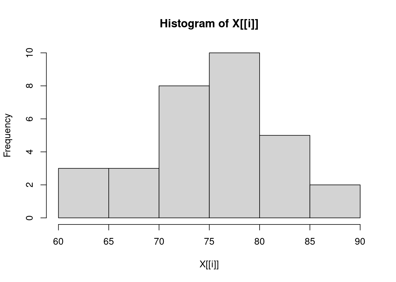
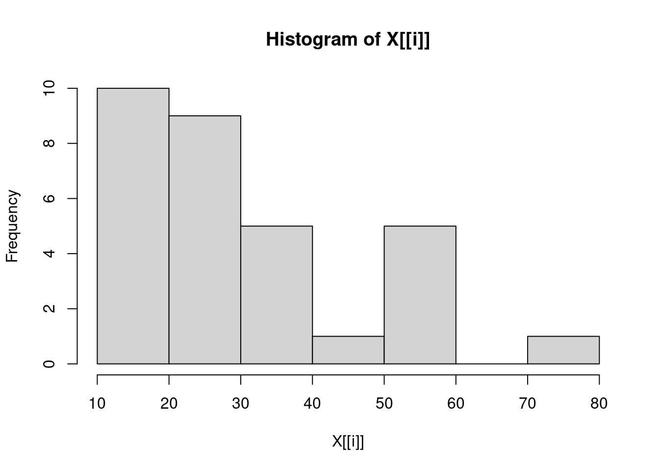
         Girth     Height    Volume
breaks   integer,8 integer,7 integer,8
counts   integer,7 integer,6 integer,7
density  numeric,7 numeric,6 numeric,7
mids     numeric,7 numeric,6 numeric,7
xname    "X[[i]]"  "X[[i]]"  "X[[i]]"
equidist TRUE      TRUE      TRUE
sapply(trees, hist)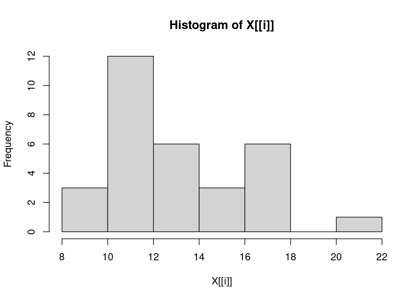


         Girth     Height    Volume
breaks   integer,8 integer,7 integer,8
counts   integer,7 integer,6 integer,7
density  numeric,7 numeric,6 numeric,7
mids     numeric,7 numeric,6 numeric,7
xname    "X[[i]]"  "X[[i]]"  "X[[i]]"
equidist TRUE      TRUE      TRUE
Problem 5
pr5_str <- "I made myself a snowball As perfect as can be I thought I’d keep it as a pet And let it sleep with me I made it some pajamas And a pillow for its head Then last night it ran away But first It wet the bed"pr5_str <- tolower(pr5_str)
str_count(pr5_str, c("a", "e", "i", "o", "u"))[1] 20 19 14 5 2str_replace_all(pr5_str, "p", "b")[1] "i made myself a snowball as berfect as can be i thought i’d keeb it as a bet and let it sleeb with me i made it some bajamas and a billow for its head then last night it ran away but first it wet the bed"Problem 6
Pascal’s Triangle arises from the coefficients of the binomial expansion \((x + y)^n\).
These are combinations \(\left(n \atop r\right) = C(n,r) = \text{choose}(n,r)\) in R.
Problem 6a
Create the following list
list_6 <- list(c(1), c(1, 1), c(1, 2, 1), c(1, 3, 3, 1))list(1, choose(1, 0:1), choose(2, 0:2), choose(3, 0:3))[[1]]
[1] 1
[[2]]
[1] 1 1
[[3]]
[1] 1 2 1
[[4]]
[1] 1 3 3 1pascals_func <- function(n){
#setting up a list with a 1 at the start.
ret_val <- list()
ret_val[1] <- 1
# i will function as a variable and counter simultaneously!
i <- 1
while (i <= n){
# Set x to the list output of the choose function. This breaks if "list" is not specified.
x <- list(choose(i, 0:i))
# append x to ret_val
ret_val <- append(ret_val, x)
# increments i up by 1 with every loop. Caps at n+1.
i <- i + 1
}
return(ret_val)
}pascals_func(5)[[1]]
[1] 1
[[2]]
[1] 1 1
[[3]]
[1] 1 2 1
[[4]]
[1] 1 3 3 1
[[5]]
[1] 1 4 6 4 1
[[6]]
[1] 1 5 10 10 5 1pascals_func(10)[[1]]
[1] 1
[[2]]
[1] 1 1
[[3]]
[1] 1 2 1
[[4]]
[1] 1 3 3 1
[[5]]
[1] 1 4 6 4 1
[[6]]
[1] 1 5 10 10 5 1
[[7]]
[1] 1 6 15 20 15 6 1
[[8]]
[1] 1 7 21 35 35 21 7 1
[[9]]
[1] 1 8 28 56 70 56 28 8 1
[[10]]
[1] 1 9 36 84 126 126 84 36 9 1
[[11]]
[1] 1 10 45 120 210 252 210 120 45 10 1Problem 7.
Import the built-in data set “iris”.
Problem 7a
Using the original data frame, compute the mean and standard deviation of the petal lengths.
cat("The mean of the petal length in iris is", round(mean(iris$Petal.Length), digits = 2), "\n")The mean of the petal length in iris is 3.76 cat("The standard deviation of the petal length in iris is", round(sd(iris$Petal.Length), digits = 2), "\n")The standard deviation of the petal length in iris is 1.77 Problem 7b
Compute the maximum petal width and maximum petal length.
cat("The max petal width is", max(iris$Petal.Width), "\n")The max petal width is 2.5 cat("The max petal length is", max(iris$Petal.Length), "\n")The max petal length is 6.9 Problem 7c
Extract the rows corresponding the species iris versicolor flowers and save it to a new data frame “VersicolorIris”.
VersicolorIris <- subset(iris, Species == "versicolor")Problem 7d
Compute the mean and standard deviation of the Versicolor petal lengths
cat("The mean petal length of the versicolor iris is", mean(VersicolorIris$Petal.Length), "\n")The mean petal length of the versicolor iris is 4.26 cat("The standard deviation of the versicolor iris is", round(sd(VersicolorIris$Petal.Length), digits = 2), "\n")The standard deviation of the versicolor iris is 0.47 Problem 7e
Extract the Species and Petal Length columns and save to a new data frame ‘Petal-Length’.
# I'll be using select() from the tidyverse package here. It's so convenient.

data_7e <- as_tibble(iris)

Petal_Length <- data_7e %>% select(Petal.Length, Species)
unstack(Petal_Length)
setosa versicolor virginica
1 1.4 4.7 6.0
2 1.4 4.5 5.1
3 1.3 4.9 5.9
4 1.5 4.0 5.6
5 1.4 4.6 5.8
6 1.7 4.5 6.6
7 1.4 4.7 4.5
8 1.5 3.3 6.3
9 1.4 4.6 5.8
10 1.5 3.9 6.1
11 1.5 3.5 5.1
12 1.6 4.2 5.3
13 1.4 4.0 5.5
14 1.1 4.7 5.0
15 1.2 3.6 5.1
16 1.5 4.4 5.3
17 1.3 4.5 5.5
18 1.4 4.1 6.7
19 1.7 4.5 6.9
20 1.5 3.9 5.0
21 1.7 4.8 5.7
22 1.5 4.0 4.9
23 1.0 4.9 6.7
24 1.7 4.7 4.9
25 1.9 4.3 5.7
26 1.6 4.4 6.0
27 1.6 4.8 4.8
28 1.5 5.0 4.9
29 1.4 4.5 5.6
30 1.6 3.5 5.8
31 1.6 3.8 6.1
32 1.5 3.7 6.4
33 1.5 3.9 5.6
34 1.4 5.1 5.1
35 1.5 4.5 5.6
36 1.2 4.5 6.1
37 1.3 4.7 5.6
38 1.4 4.4 5.5
39 1.3 4.1 4.8
40 1.5 4.0 5.4
41 1.3 4.4 5.6
42 1.3 4.6 5.1
43 1.3 4.0 5.1
44 1.6 3.3 5.9
45 1.9 4.2 5.7
46 1.4 4.2 5.2
47 1.6 4.2 5.0
48 1.4 4.3 5.2
49 1.5 3.0 5.4
50 1.4 4.1 5.1Problem 8: THE BIRTHDAY PROBLEM
What is the probability that in a set of \(n\) randomly selected people at least two people have the same birthday?
If we have a group of 366 (or 367 for a leap year), there is a 100% probability that two people have the same birthday.
How many people do you need so that the probability is at least 50%? It is surprising to learn that only 23 people are needed for a 50% chance of two people with the same birthday. And if there are 60 people in the room, the probability increases to 99.41%.
The probability is given by the formula:
\[p(n) = 1 - \frac{365!}{365^n (365 - n)}\]
Problem 8a
birthday <- function(n){
  1 - prod(seq(from=1, to = (365 - n + 1) / 365, by = -1/365))
}
BdayProb <- sapply(1:70, birthday)
Problem 8b
plot(1:70, BdayProb, pch = 20, xlab = "Number of People", ylab = "Probability")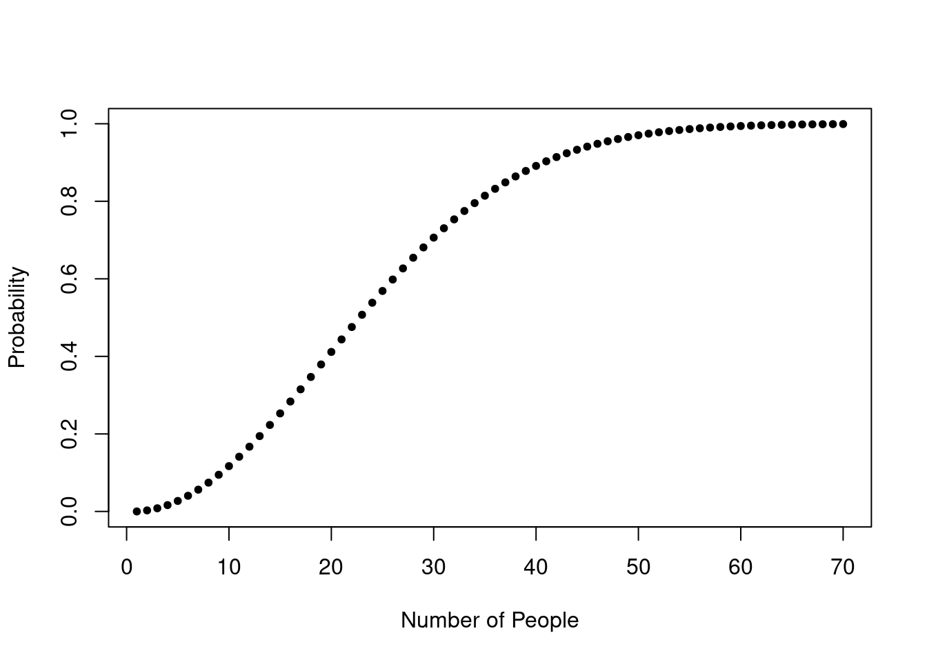
Problem 8d
Create a nicer plot. Run the following code.
library(reshape)
library(ggplot2)

# Input the value for npeople. Change this value to change the graph.
  npeople = 70

# Create a data frame Bday using the birthday function
  Bday = data.frame(n = 1:npeople, ProbTwoSame =
    sapply(1:npeople, birthday), y = 0.5)

  # Melt the data for casting (Smooths the data points)
  Bday = reshape::melt(Bday, id.vars = "n")

  ggplot(Bday, aes(x = n, y = value, colour = variable)) + geom_line() + scale_colour_hue("") + xlab("Number of People") + ylab("Probability")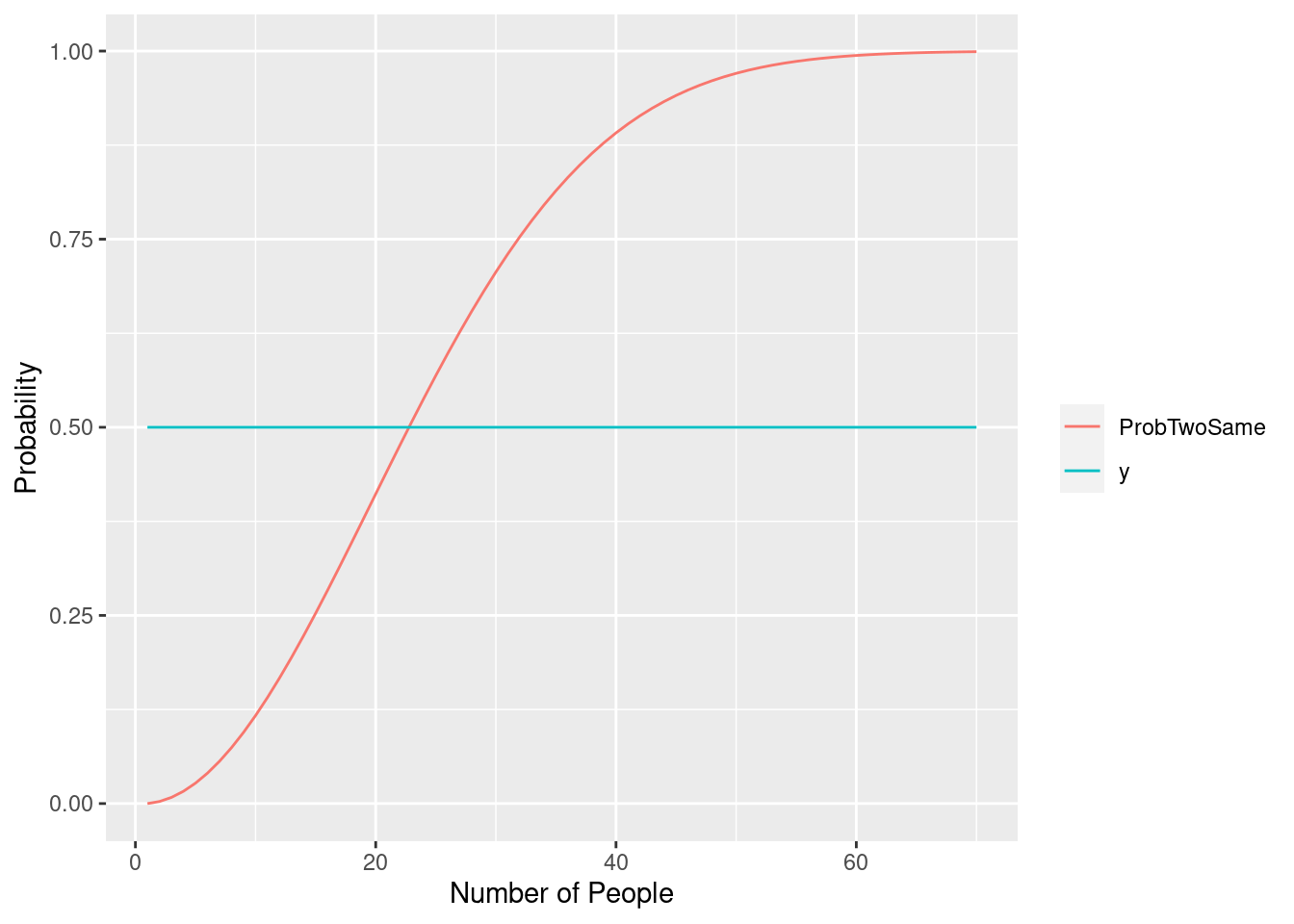
I believe I got this working correctly. I ran into an issue where “+” was on a new line, so making it one giant gnarly line got it at least compiling.