MTH-2520 Homework 9: Graphing with Base R

Problem 1.

Load in the colorado covid-19 stats taken from the Colorado Department of Public Health and Environment.

covid <- read.csv("CO_COVID19.csv")

Problem 1a

Compute summary statistics for the daily number of cases and the daily number of deaths.

summary(covid$DailyCases)

##    Min. 1st Qu.  Median    Mean 3rd Qu.    Max. 
##      33     324     576    1216    1541    6439

summary(covid$DailyDeaths)

##    Min. 1st Qu.  Median    Mean 3rd Qu.    Max. 
##  -10.00    3.00    9.00   16.29   20.00  267.00

Problem 1b

Draw a boxplot for the cumulative number of cases.

boxplot(covid$CumulativeCases, main="Cumulative Covid Cases",
        xlab="Number of Cases", horizontal=TRUE, col = "blue")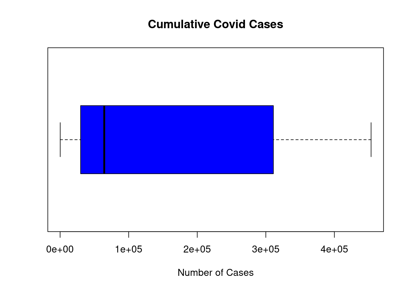

Problem 1c

Draw a boxplot for the cumulative number of deaths.

boxplot(covid$CumulativeDeaths, main="Cumulative Covid Deaths",
        xlab="Number of Deaths", horizontal=TRUE, col = "red")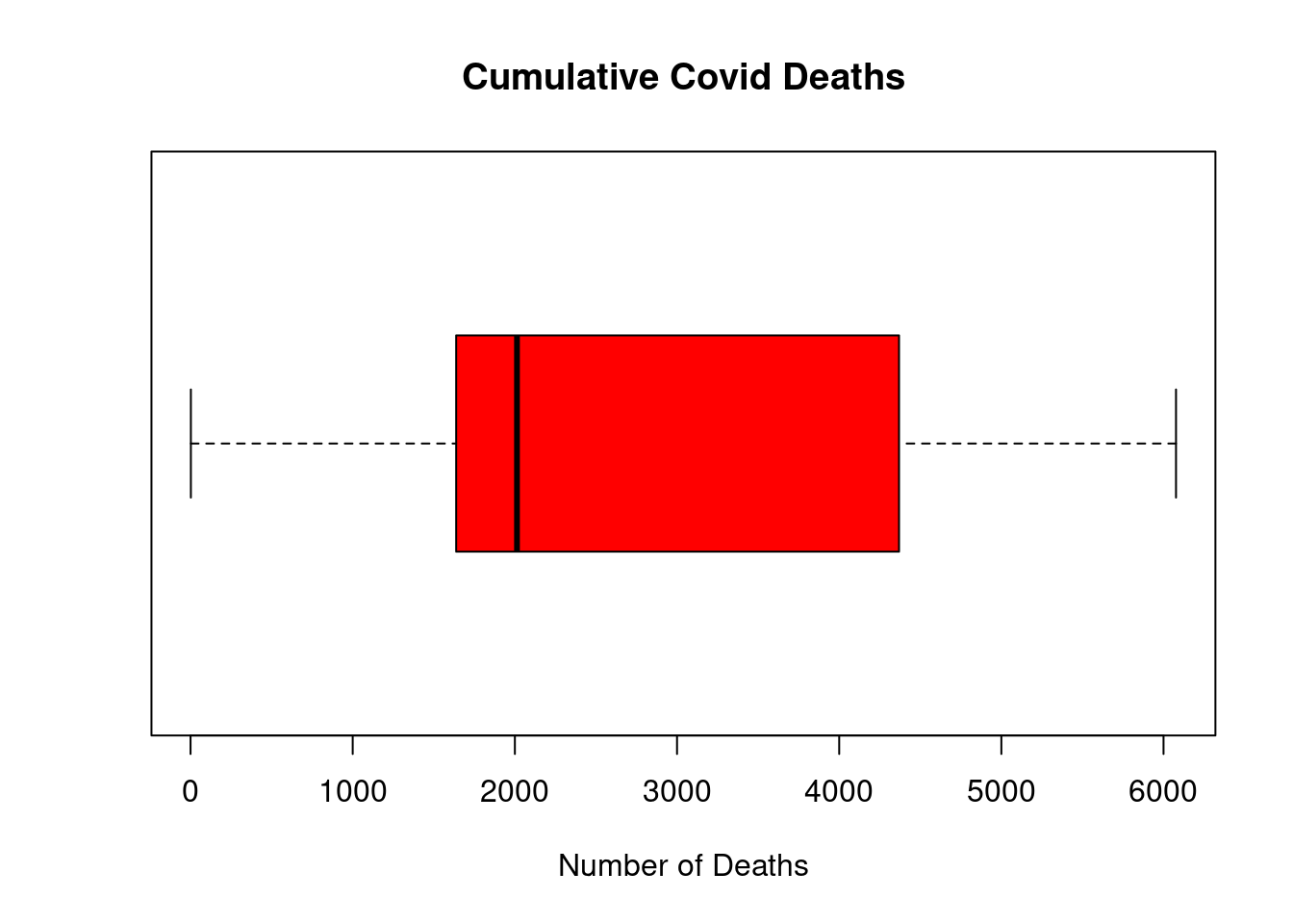

Problem 1d

Draw a time series plot for the daily number of cases.

covid_cases <- ts(covid$DailyCases, start = 1, end = 373, frequency=1)
# This feels a little hacky but it mostly works. 
class(covid_cases)

## [1] "ts"

plot(covid_cases, type = "l")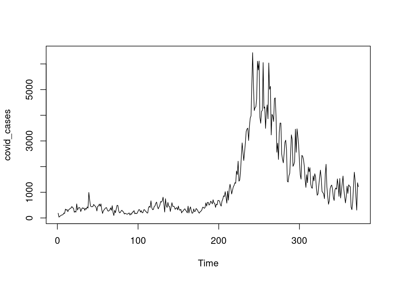

Problem 1e

Draw a time series plot for the daily number of deaths.

covid_deaths <- ts(covid$DailyDeaths, start = 1, end = 373, frequency=1)
plot(covid_deaths, type = "l")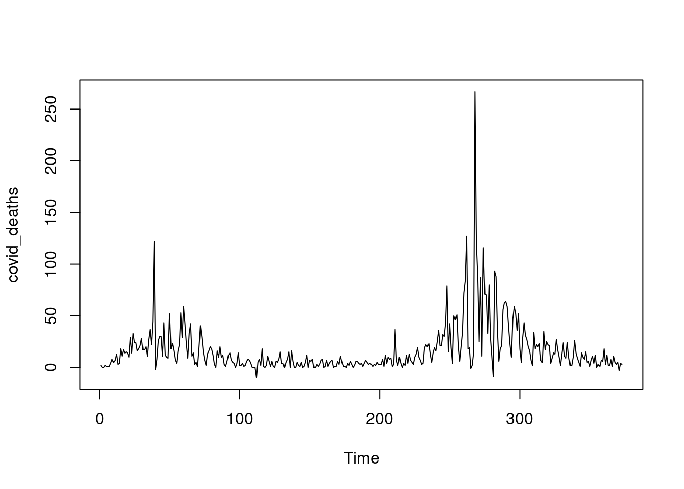

Problem 1f

Draw a scatterplot of the daily number of cases versus the daily number of deaths.

# Read in the data
covid19 <- read.csv("CovidMonthlyData.csv")

# Plot the data
plot(covid19$Cases, covid19$Deaths, main = "Daily Cases vs. Daily Deaths", 
     xlab="Cases", ylab="Deaths")
abline(lm(covid19$Deaths ~ covid19$Cases), col = "red", lwd=2)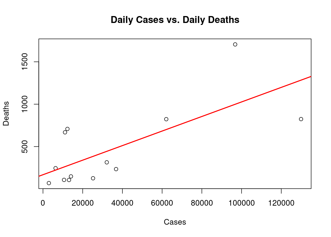

Problem 1g

Draw a bar graph for the monthly number of cases.

barplot(covid19$Cases, names=covid19$Date, xlab= "Month", ylab = "# of cases", 
        col = "pink", main ="Monthly Cases", border="black")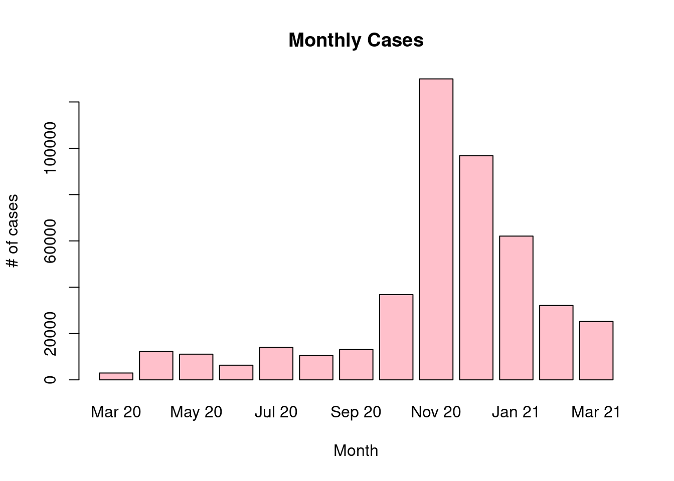

Problem 1f

Draw a bar graph for the monthly number of deaths.

barplot(covid19$Deaths, names=covid19$Date, xlab= "Month", ylab = "# of deaths", 
        col = "yellow", main ="Monthly Deaths", border="black")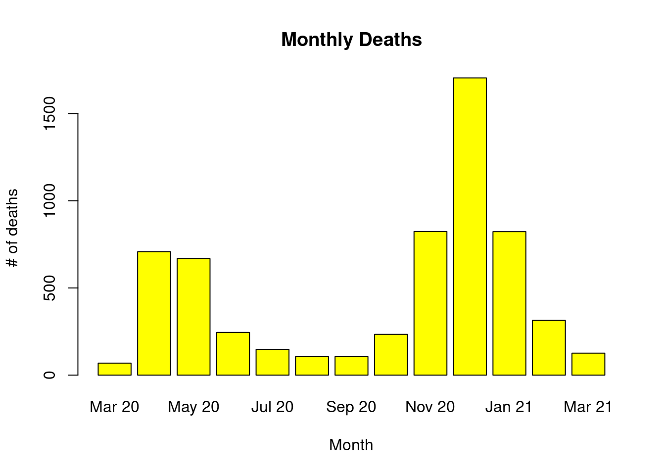

Problem 1i

Draw a pie chart for the monthly number of cases

pie(covid19$Cases, labels = covid19$Date, main = "Covid19 Cases by Month", radius = 1)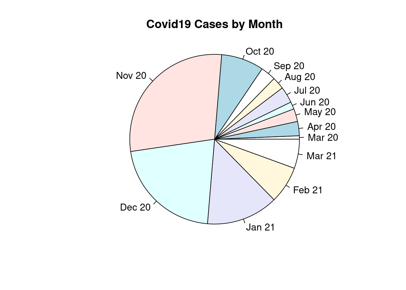

Problem 1j

Draw a pie chart for the monthly number of deaths.

pie(covid19$Deaths, labels = covid19$Date, main = "Covid19 Deaths by Month", radius = 1)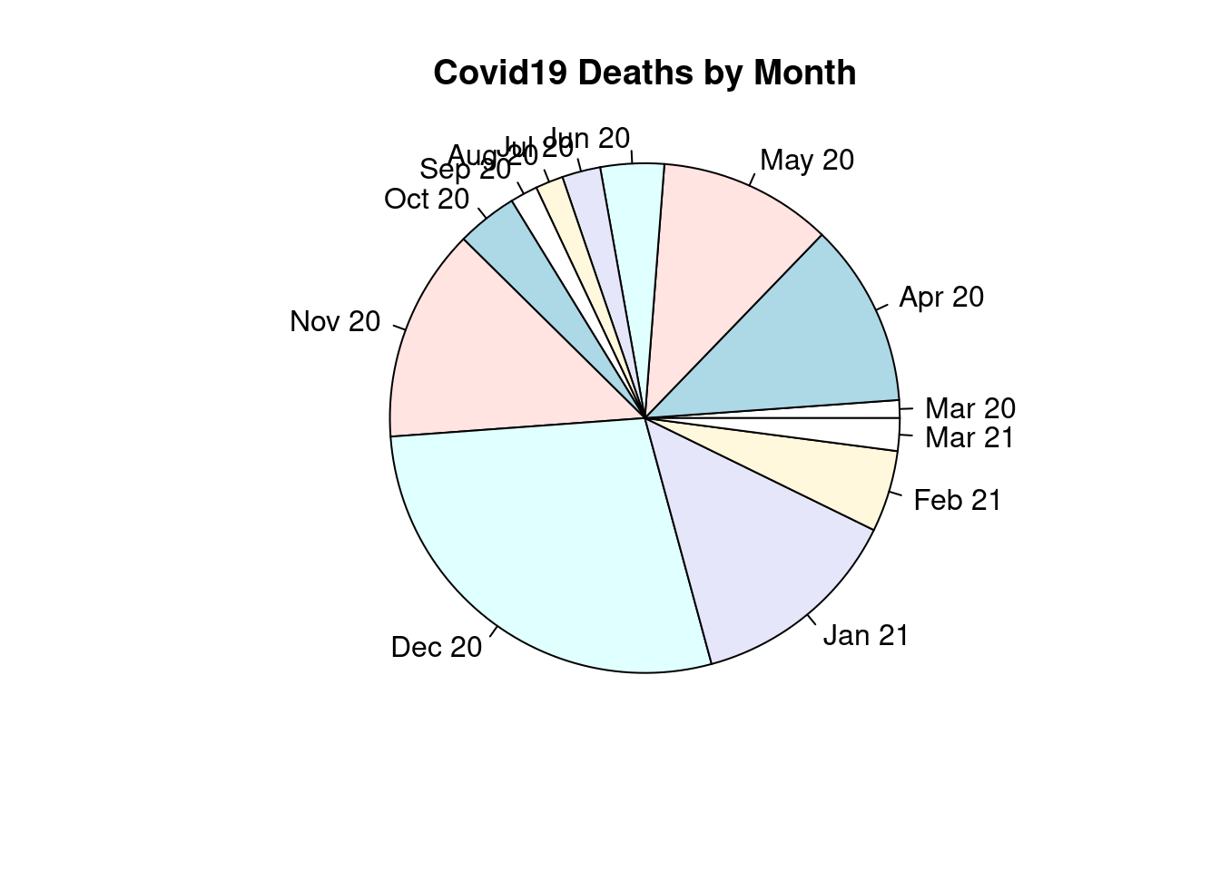

These poor pie charts are so smushed together. Hopefully ggplot pie charts are a little more robust.

Problem 2

Graph the following functions.

Problem 2a

\[f(x) = \frac{2x}{x^2 - x - 6} \; \text{on} \; [-7, 7]\]

x <- seq(-7, 7, 1)
y <- ((2 * x) / (x^2 - x - 6))
plot(x, y, pch=5, type="l")
abline(v=0, h=0)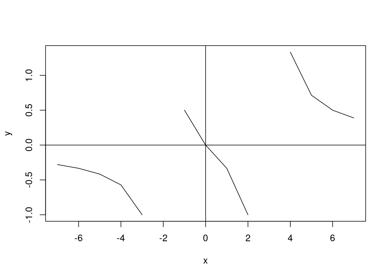

This plot is really trying to be what it’s supposed to be. I have to commend it for the effort at the very least.

Problem 2b

\[ f(x) = \begin{cases} sin(x), & x < 0 \\ 0.5x + 2, & x \geq 0 \\ \end{cases} \]

x <- seq(-10, 10, 1)
y <- function(x) {
  ifelse( 
    (x < 0), sin(x), 
    ifelse(
      (x >= 0), (0.5 * x + 2), NA)
  )}

plot(y, xlim = c(-10, 10), ylim = c(-2, 5), col="red", lwd=2)
abline(v=0, h=0)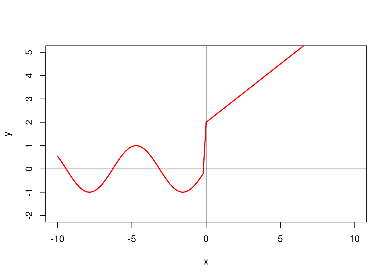

Problem 3

Run the following code.

t <- seq(from=0, to=12*pi, by=0.001)
x <- 4.5*sin(t) - sin(3*t) + 0.8*sin(15.25*t)
y <- 4*cos(t) - 1.5*cos(2*t) - 0.6*cos(3*t) - 0.3*cos(4*t) + 0.8*cos(15.25*t)
plot(x, y, type = "l", lwd = 2, col = "red", xlab = "", ylab = "", axes = FALSE)

Problem 4 [Parametric Equations]

Lissajous or Bowditch curves. \[x = A \sin(\alpha t + \delta), \; y = B \sin(bt) \; \text{on} \; [0, 2\pi]\]

Graph two (or more) Lissajous curves for different values of \(A, B, a, b, \delta\).

lissajous <- function(A, B, alpha, beta, delta, color){
  t <- seq(0, 2*pi, 0.01)
  x <- A*sin(alpha * t + delta)
  y <- B*sin(beta * t)
  
  plot(x, y, type = "l", col = color, main = "Lissajous Curve", lwd = 2)
}

lissajous(A=1, B=1, alpha=2, beta=3, delta=0, "purple")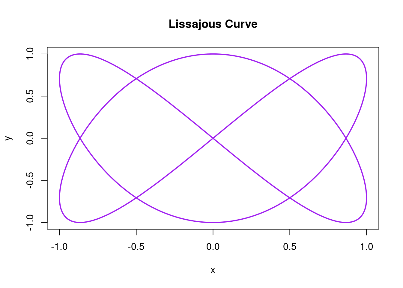

lissajous(A=2, B=1, alpha=3, beta=5, delta=2, "red")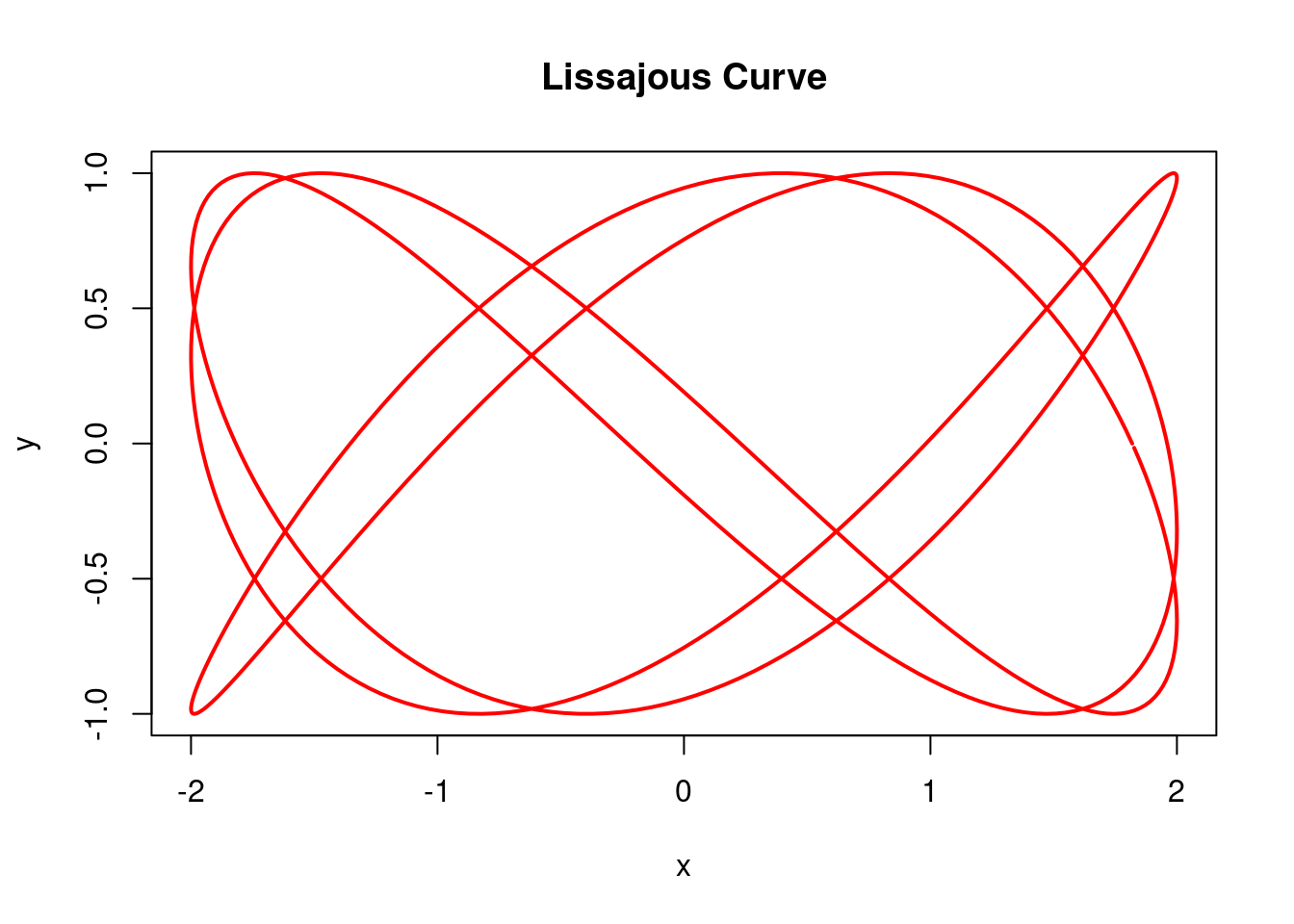

lissajous(A=7, B=3, alpha=20, beta=4, delta=7, "green")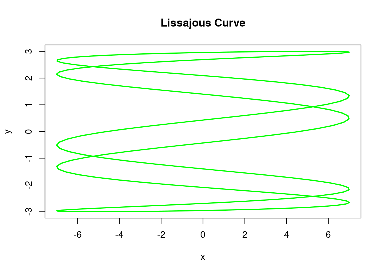

Problem 5 [Parametric Graphs]

Problem 5a

Write a function Parametric(B, r, color) that will plot the following graphs given the period B, the function r, and a color such as “red”.

# So I accidentally already made a function nearly identical to this. So we'll take that and very slightly tweak it to match. Mine was a little gnarly with how many arguments it took in anyhow. 

Parametric <- function(B, r, color){
  t <- seq(0, B, 0.001)
  x <- r*cos(t)
  y <- r*sin(t)
  
  plot(x, y, type = "l", lwd = 2, col = color, xlab = "",
  ylab = "", axes = FALSE)
}

Problem 5b

Graph the following using your function.

# b1
Parametric(B=(2*pi), r=(1+4*cos(5*t)), color="red")

## Warning in r * cos(t): longer object length is not a multiple of shorter object
## length

## Warning in r * sin(t): longer object length is not a multiple of shorter object
## length

# b2
Parametric(B=(2*pi), r=(1+4*cos(10*t)), color="purple")

## Warning in r * cos(t): longer object length is not a multiple of shorter object
## length

## Warning in r * sin(t): longer object length is not a multiple of shorter object
## length

# b3
Parametric(B=(10*pi), r=(sin((2*t)/5)), color="green")

## Warning in r * cos(t): longer object length is not a multiple of shorter object
## length

## Warning in r * sin(t): longer object length is not a multiple of shorter object
## length

# b4
Parametric(B=(10*pi), r=(sin((4*t)/5)), color="green")

## Warning in r * cos(t): longer object length is not a multiple of shorter object
## length

## Warning in r * sin(t): longer object length is not a multiple of shorter object
## length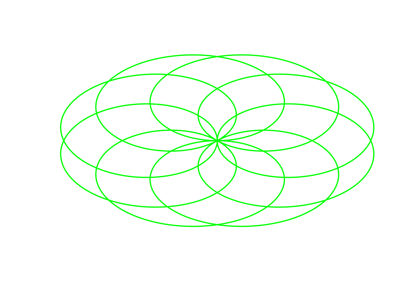

# b5
Parametric(B=(10*pi), r=(sin((8*t)/5)), color="black")

## Warning in r * cos(t): longer object length is not a multiple of shorter object
## length

## Warning in r * sin(t): longer object length is not a multiple of shorter object
## length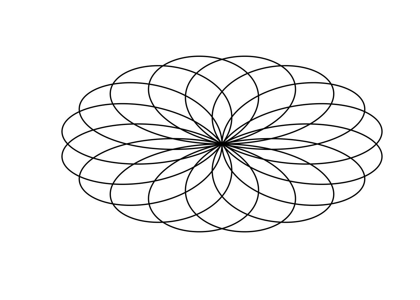

# b6
Parametric(B=(12*pi), r=(2 - 5*sin(t/6)), color="black")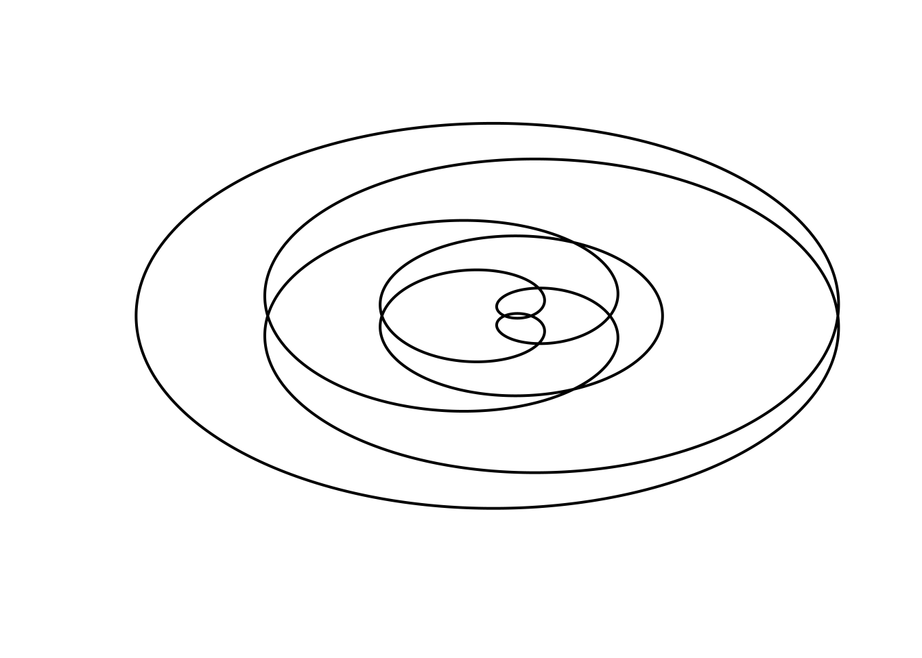

# b7
Parametric(B=(12*pi), r=(2 - 5*sin(5*t/6)), color="black")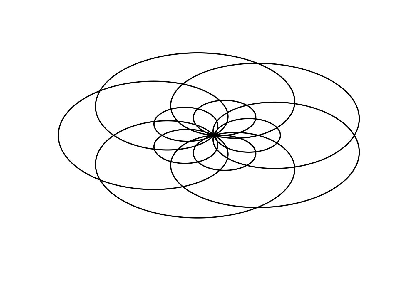

# b8
Parametric(B=(2*pi), r=(exp(1)^(cos(t)) - 2*cos(4*t)), color="purple")

## Warning in r * cos(t): longer object length is not a multiple of shorter object
## length

## Warning in r * sin(t): longer object length is not a multiple of shorter object
## length

# b9
Parametric(B=(2*pi), r=(exp(1)^(cos(t)) - 2*cos(4*t) + sin(t/12)^5), color="red")

## Warning in r * cos(t): longer object length is not a multiple of shorter object
## length

## Warning in r * sin(t): longer object length is not a multiple of shorter object
## length

# b10_1
Parametric(B=(20*pi), r=(17 - 12*sin(20*t/12)), color="black")

## Warning in r * cos(t): longer object length is not a multiple of shorter object
## length

## Warning in r * sin(t): longer object length is not a multiple of shorter object
## length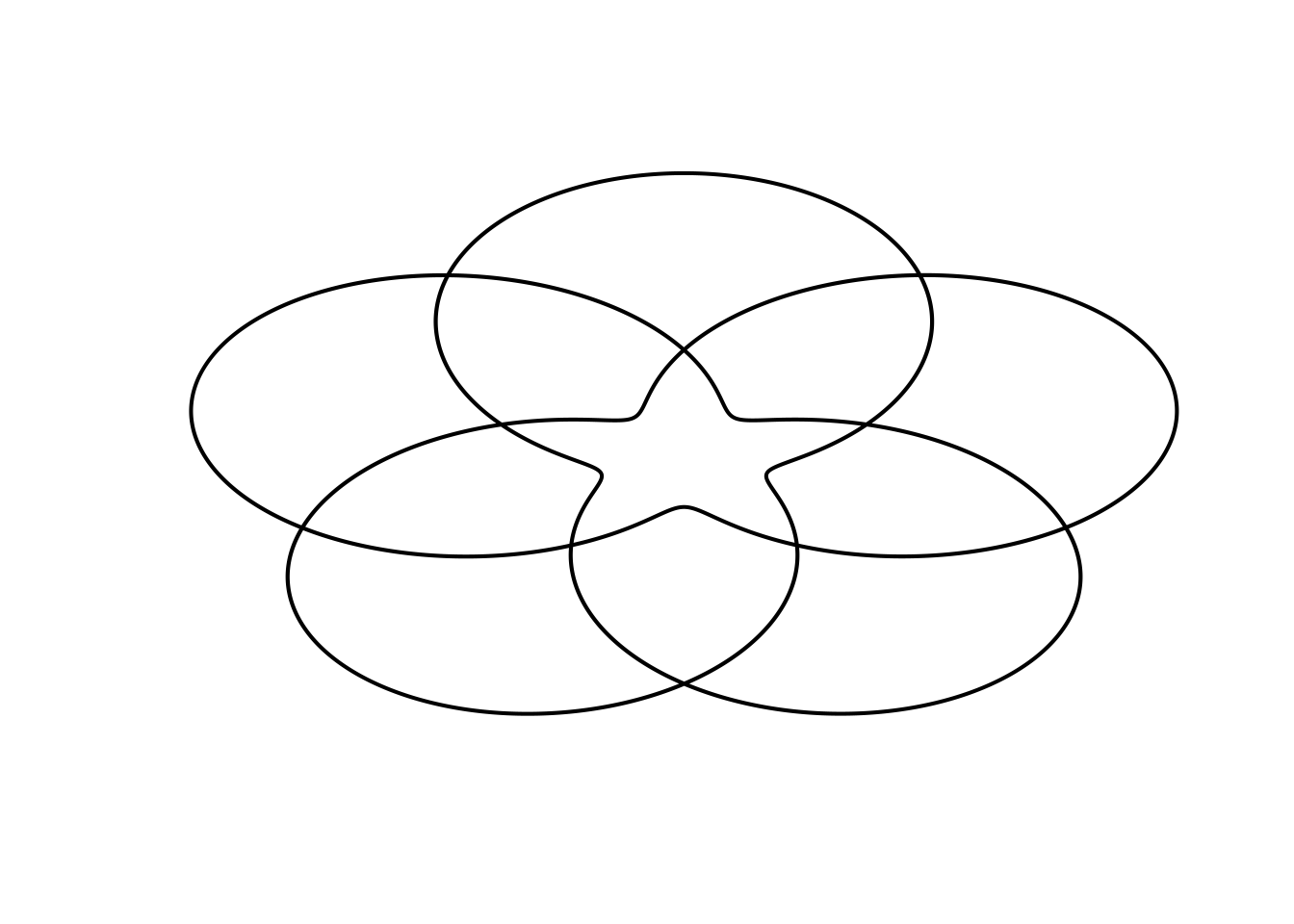

# b10_2
Parametric(B=(3*pi), r=(3 - 5*sin(5*t/6)), color="black")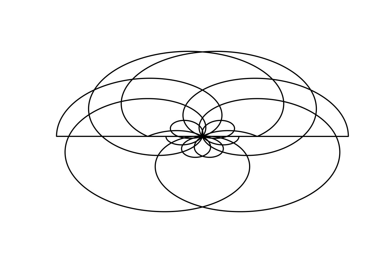

Problem 6 [Epicycloids]

An epicycloid is the curve that is traced out by a fixed point on a circle of radius r when this circle is rolled around a circle of radius \(R\).

The parametric equations for the epicycloid on \([0, (R + r)\pi]\) are:

\[x = (R + r) \cos t - r \cdot \cos \left( \frac{R + r}{r} \cdot t \right)\] \[y = (R + r) \sin t - r \cdot \sin \left( \frac{R + r}{r} \cdot t \right)\]

Problem 6a

Write a function Epicycloid(r, R) that will plot the epicycloid.

Epicycloid <- function(r, R){
  t <- seq(from=0, to=(R + r)*2*pi, len=10000)
  
  x <- (R + r)*cos(t) - (r * cos(((R+r)/r)*t))
  # print(x)
  
  y<- (R + r)*sin(t) - (r * sin(((R+r)/r)*t)) 
  # print(y)
  
  plot(x, y, type = "l", lwd = 2, )
  }

Epicycloid(r=1, R=1)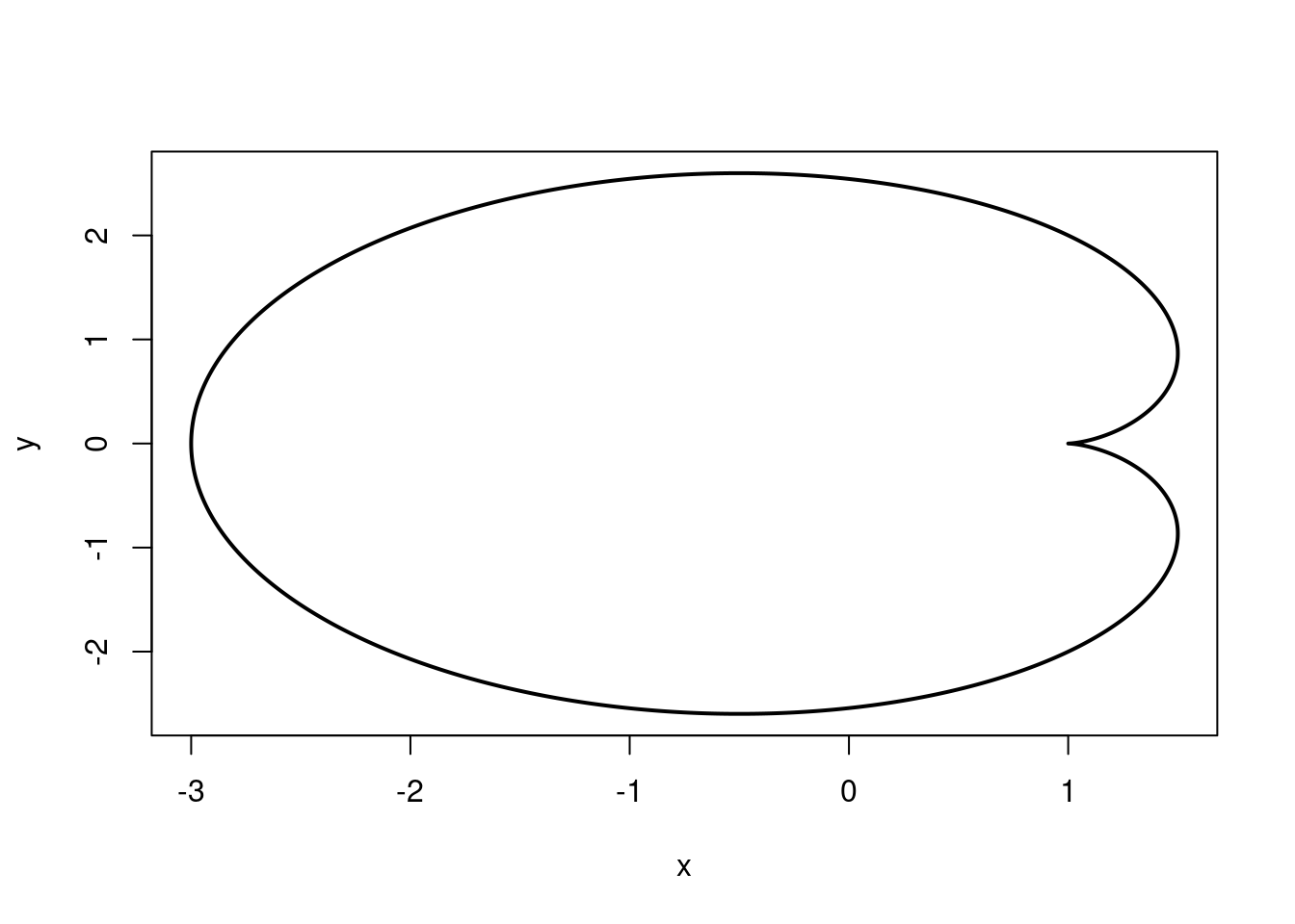

Epicycloid(r=1, R=2)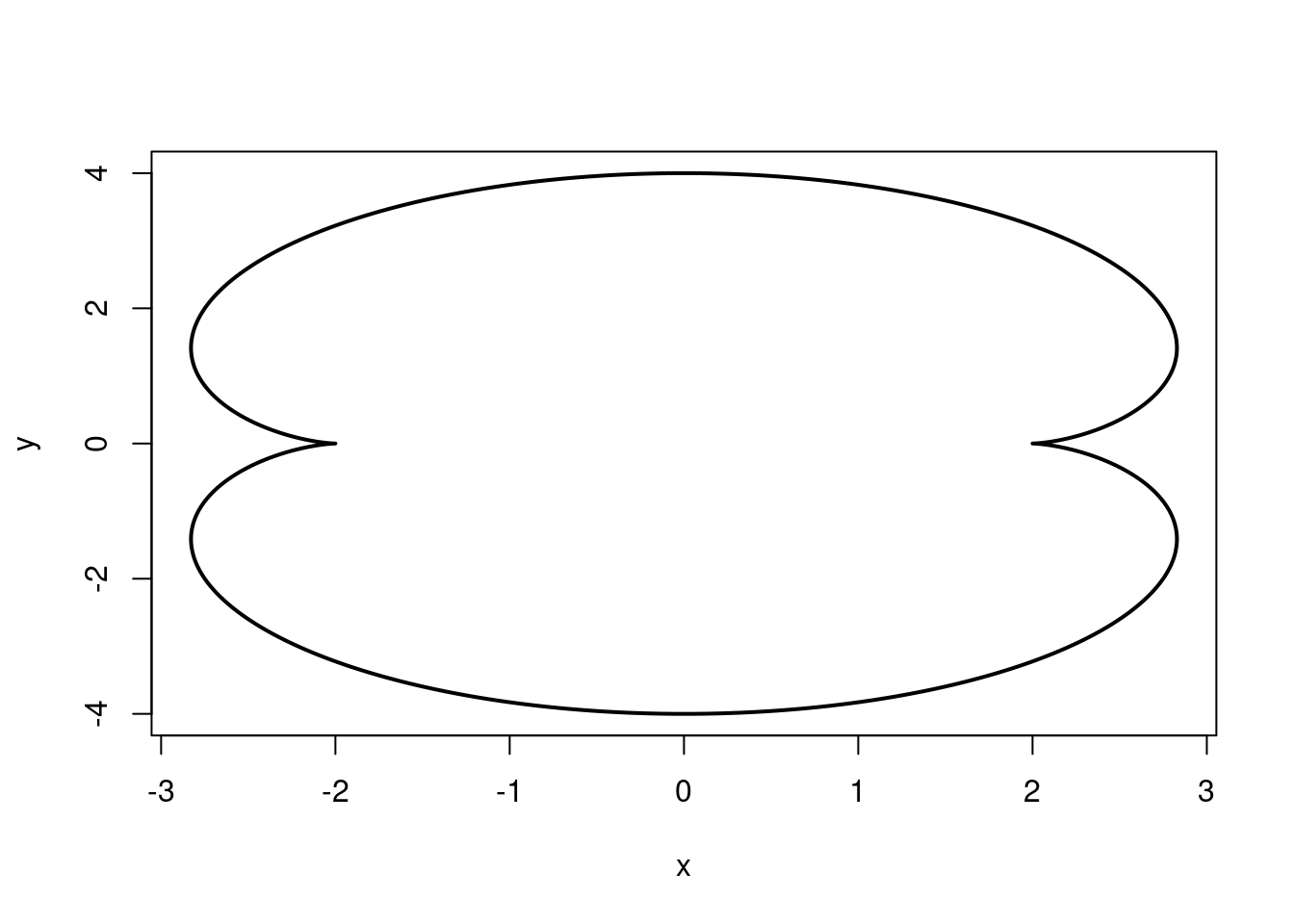

Epicycloid(r=1, R=4)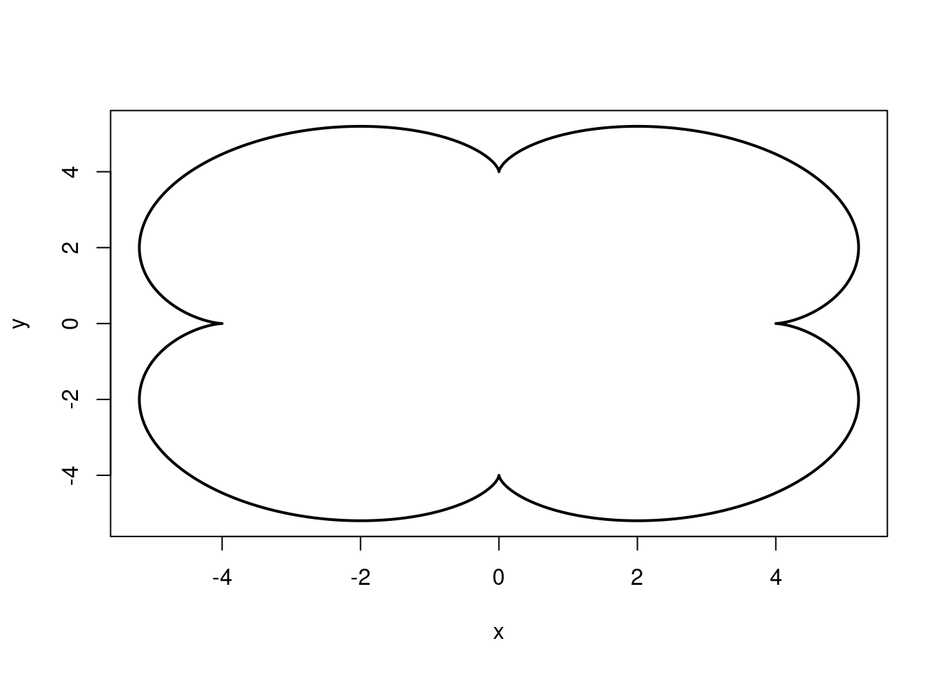

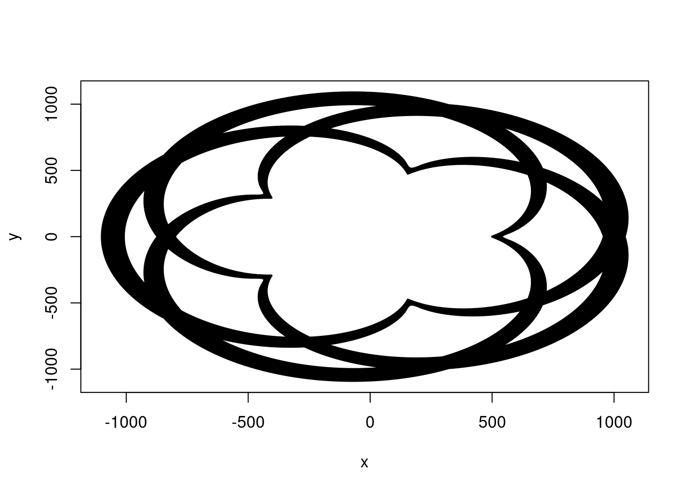
Epicycloid(r=6, R=5)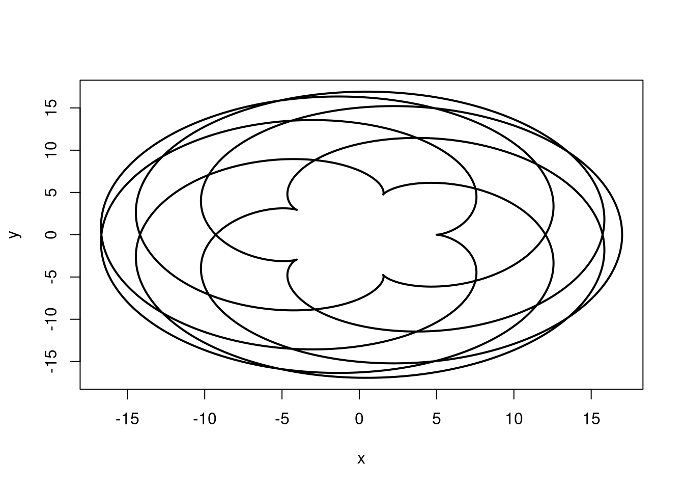

Epicycloid(r=10, R=21)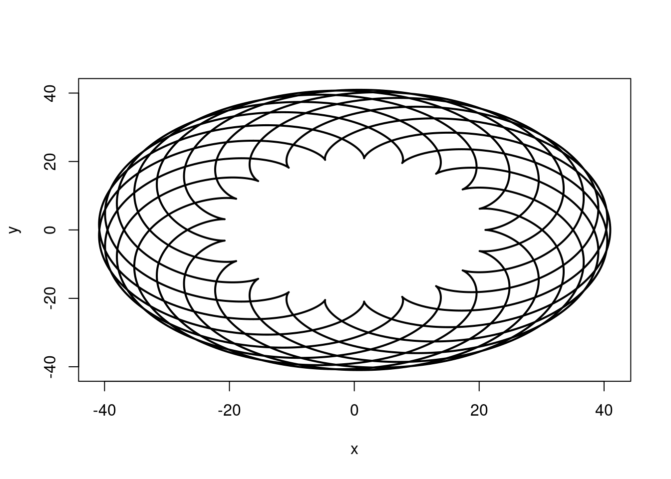

Epicycloid(r=15, R=20)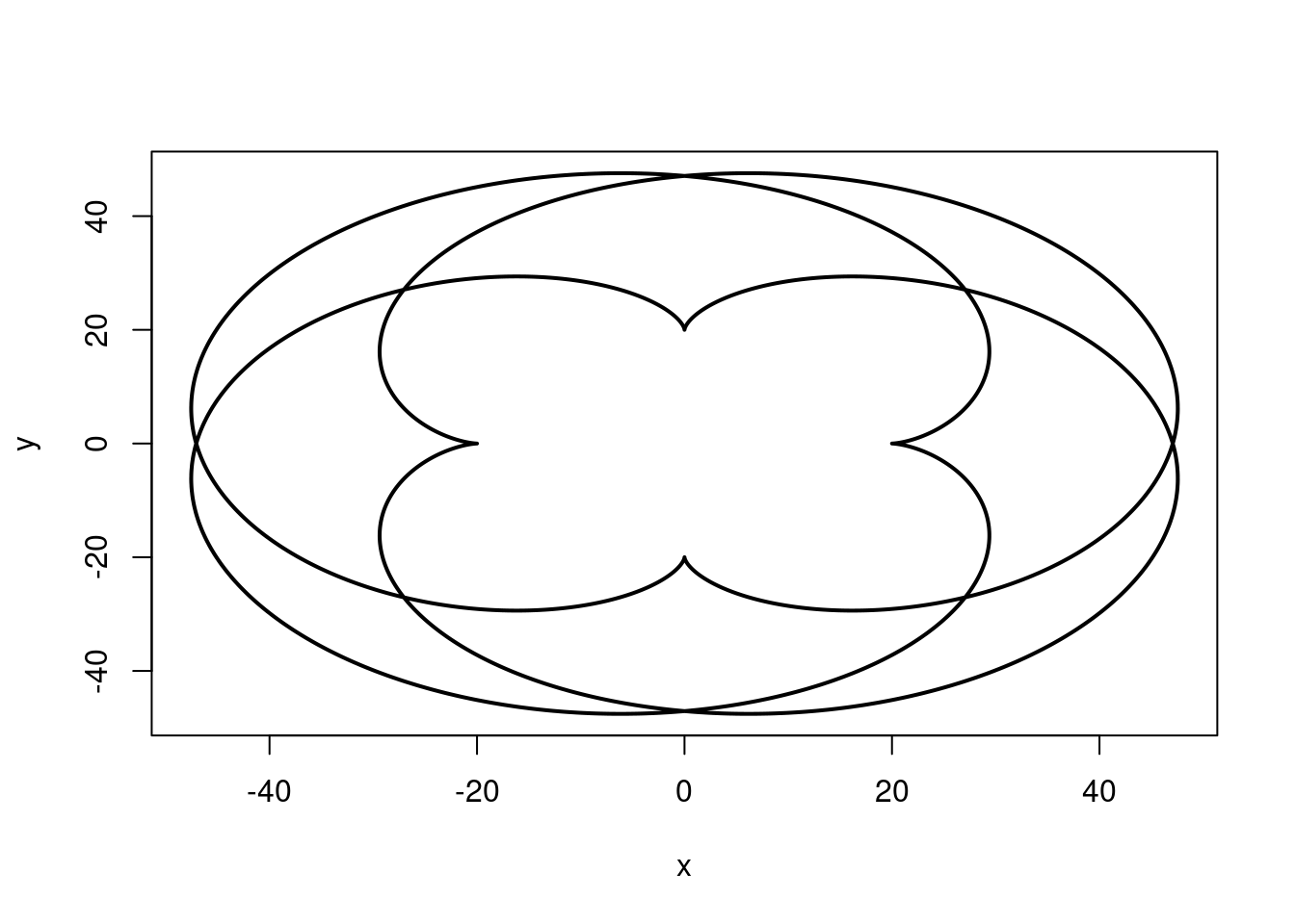

Epicycloid(r=300, R=500)