Simple Random Sample
Poet: Stephen Crane
Source: Poems of Stephen Crane (Selected by Gerald D. McDonald (1964))
Population: All poems written by Stephen Crane.
Note that it is likely the selected book does not contain every single poem from this poet.
Total number of poems: 59 poems (index starting at 1, the poem number is just the page in the book)
Method:
Let x be a random positive integer such that:
\[1\leq x \leq 59\]
This selects the poem. From there, count number of lines.
Let y be a random number such that:
\[1 \leq y \leq n\]
where n is the number of lines.
From here the syllables on line y are counted.
Generate our poem list.
The below code was ran to generate our list of poems. It is now commented out.
#sample.int(59, 30, replace = TRUE)The list generated by this code is provided below and saved.
poem_list <- c(26, 34, 53, 16, 34, 57, 12, 35, 46, 9, 43, 17, 23, 39, 3, 39, 49, 11, 56,
               58, 20, 59, 25, 46, 41, 21, 23, 2, 20, 11)
Now this is where things get a bit more tedious. As a physical book is being used, for each of these poems the number of lines must be found manually. The random number y will be generated one at a time due to the nature of line-counting.
The first randomly selected poem will serve as an example. The number is 26, which indicates our first poem is “I explain the silvered passing” on page 26. This poem has a total of 13 lines.
#sample.int(13, 1)sample.int(13,1) gave us the number 4. Line 4 has 10 syllables. This system will be used for the remaining 29 poems.
This system guarantees that all poems have equal chance of being selected instead of longer poems having a higher chance. At least, that was the intent. A bias in this system arose when it was realized that there was a single poem that took up two pages. This, of course, means that it is more likely than the rest to be selected. Another issue encountered was that some of the stanza lines were too long for the books margins and had one word on a second line. These longer stanza lines were considered a single line for the sake of the experiment. An example of this choice is provided from the first paragraph of a poem below:
- “There were many who went in huddled
procession,
- They knew not whither;
- But, at any rate, success or calamity
- Would attend all in equality.”
(There were many who went, Stephen Crane)
This is not a perfect solution as it is difficult to maintain consistency with this methodology. Care was taken to ensure consistency with the lines that were combined. Understand this may skew the average to be higher.
Below is a list of the collected syllable counts and the resulting summary statistics.
syllable_sample_one <- c(10,8,8,8,7,7,4,12,6,5,8,10,7,8,5,11,8,11,7,8,4,8,4,4,9,11,7,4,11,3)
syllable_sample_two <- c(2,6,4,7,4,3,4,5,3,4,4,4,4,8,6,6,7,4,2,4,7,6,2,4,2,6,4,10,3,5)

cat("The sample standard deviation for sample one is:", round(sd(syllable_sample_one),2),
    "Syllables \n \n")
## The sample standard deviation for sample one is: 2.51 Syllables
## cat("The sample standard deviation for sample two is:", round(sd(syllable_sample_two),2),
"Syllables \n \n")## The sample standard deviation for sample two is: 1.92 Syllables
## cat("The summary statistics for sample one are: \n")## The summary statistics for sample one are:summary(syllable_sample_one)## Min. 1st Qu. Median Mean 3rd Qu. Max.
## 3.000 5.250 8.000 7.433 8.750 12.000cat("\nThe summary statistics for sample two are: \n")##
## The summary statistics for sample two are:summary(syllable_sample_two)## Min. 1st Qu. Median Mean 3rd Qu. Max.
## 2.000 4.000 4.000 4.667 6.000 10.000boxplot(syllable_sample_one, syllable_sample_two,
horizontal = TRUE,
xlab = "Line Length (Syllables)",
names = c("Stephen Crane", "Partner Sample"))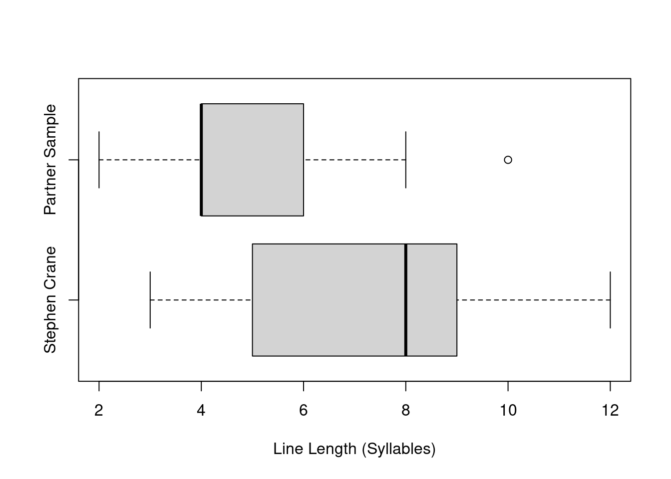
Frequency Table:
| # Of Syllables | Frequency | Relative Frequency |
|---|---|---|
| 1 | 0 | 0 |
| 2 | 0 | 0 |
| 3 | 1 | \(1/30 \approx .033\) |
| 4 | 5 | \(5/30 \approx .167\) |
| 5 | 2 | \(2/30 \approx .067\) |
| 6 | 1 | \(1/30 \approx .033\) |
| 7 | 5 | \(5/30 \approx .167\) |
| 8 | 8 | \(8/30 \approx .267\) |
| 9 | 1 | \(1/30 \approx .033\) |
| 10 | 2 | \(2/30 \approx .067\) |
| 11 | 4 | \(4/30 \approx .133\) |
| 12 | 1 | \(1/30 \approx .033\) |
syllable_df_one = as.data.frame(syllable_sample_one)
ggplot(data = syllable_df_one, aes(x=syllable_sample_one, y = ..count../sum(..count..))) +
  geom_histogram(binwidth = 1, colour = 'black') +
  labs(title = "Relative Frequency Histogram of Stephen Crane Poem Line Lengths",
       subtitle = "Poems Selected by Gerald D. McDonald (1964)") +
  scale_x_continuous("Line Length (Syllables)", breaks = 3:12, labels = 3:12) +
  scale_y_continuous("Rel. Frequency", breaks = seq(0,.4,.05)) +
theme_grey() 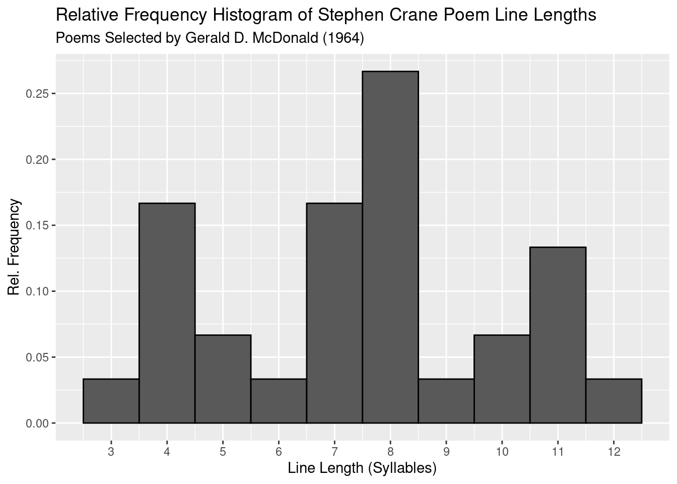
The frequency histogram for Stephen Crane does not appear to show a normal distribution. What’s noticeable is four lengths that are substantially more frequent than the rest. A normal distribution would show a more gradual decrease in frequency as values deviate away from the mean, but here that isn’t the case. It would likely be better to refer to this as a tri-modal or even a multi-modal distribution.
On the other hand though, it would be unwise to completely throw out the possibility that this distribution is normal. There are many distributions that are normal and look nothing like it. The analysis done here simply states that the given historgram does not appear to match what one would traditionally call normal.
syllable_df_two = as.data.frame(syllable_sample_two)
ggplot(data = syllable_df_two, aes(x=syllable_sample_two, y = ..count../sum(..count..))) +
  geom_histogram(binwidth = 1, colour = 'black') +
  labs(title = "Relative Frequency Histogram of Charles Tomlinson Poem Line Lengths") +
       # subtitle = "Poems Selected by Gerald D. McDonald (1964)") +
  scale_x_continuous("Line Length (Syllables)", breaks = 2:10, labels = 2:10) +
  scale_y_continuous("Rel. Frequency", breaks = seq(0,.4,.05)) +
theme_grey() 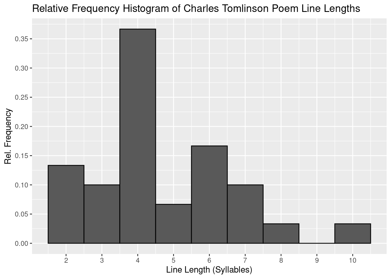
Describing this distribution as normal seems largely inaccurate. Due to the disproportionate frequency of length 4 this distribution would probably best be described as either reverse j-shaped or uni-modal and right-skewed. The same considerations from the previous histogram can be made here as well. This could definitely be a normal distribution, it just does not appear to be at a simple glance.
Data Analysis Conclusions:
Building off of the observations made in the previous section, it can be stated that both distributions are very different from each other. This goes beyond shape as well. It would be one thing if that was the main difference but it can also be seen that the Stephen Crane sample line lengths are, on average, far longer than the line length found in the second sample. This can be observed from the summary statistics and box plots which also show a far greater spread in the Stephen Crane sample. The second sample has a more dense distribution of line lengths that tend to be shorter, with a third quartile below even the median of the Stephen Crane sample.
95% Confidence Interval
lower_bound <- mean(syllable_sample_one) -
  qt(1-0.05 / 2,29) *
  sd(syllable_sample_one) / sqrt(30)

upper_bound <- mean(syllable_sample_one) +
  qt(1-0.05 / 2,29) *
  sd(syllable_sample_one) / sqrt(30)

cat("The double sided 95% confidence interval for the population mean of Stephen Crane",
      "\npoem line lengths in syllables is: \n[",
    round(lower_bound,2), ",", round(upper_bound,2), "]")
## The double sided 95% confidence interval for the population mean of Stephen Crane
## poem line lengths in syllables is:
## [ 6.49 , 8.37 ]In other words, it is known with 95% confidence that the true mean of Stephen Crane poem line lengths is between 6.49 and 8.37 syllables long based on our given sample.
Hypothesis Test
\[H_0: \mu_0 = \mu_1\] \[H_A: \mu_0 \neq \mu_1\] \[\alpha = .05\]
To put this into words, the null hypothesis is that both poets true average line length is the same. The alternative hypothesis would be the opposite, that they’re different. The significance level for this test will be 0.05. This hypothesis test will first be done with code created manually to show the step by step process, and then the built in t.test() function will be used.
First, the functions that will be used for our hypothesis test calculations are below. Functions for two sample degrees of freedom and a two sample test statistic will be used.
Degrees of freedom:
two_sample_df <- function(size1,size2,sd1,sd2, print = TRUE) {
  df_num <- ((sd1^2 / size1) + (sd2^2 / size2))^2
  df_den <- ((sd1^2 / size1)^2 / (size1-1)) + ((sd2^2 / size2)^2 / (size2-1))
  df <- floor(df_num / df_den)

  if (print == TRUE) {print(df)}

  return(df)
}
Test Statistic:
two_sample_test_statistic <- function(x_mean, y_mean, delta_null = 0,
                                      sd1, sd2, size1, size2) {
  num <- x_mean - y_mean - delta_null
  den <- sqrt((sd1^2 / size1)+(sd2^2 / size2))
  return(num/den)
}
Next, the general statistics of each sample must be calculated. The mean, sample standard deviation, and sample size will be needed from each poet.
crane_mean <- mean(syllable_sample_one)
tomlinson_mean <- mean(syllable_sample_two)
crane_sd <- sd(syllable_sample_one)
tomlinson_sd <- sd(syllable_sample_two)
crane_n <- length(syllable_sample_one)
tomlinson_m <- length(syllable_sample_two)
After these values are collected, the test statistic can be calculated and a p-value will be generated from there.
alpha = .05
test_statistic <- two_sample_test_statistic(x_mean = crane_mean, y_mean = tomlinson_mean,
                                            sd1 = crane_sd, sd2 = tomlinson_sd,
                                            size1 = crane_n, size2 = tomlinson_m)

degrees_of_freedom <- two_sample_df(size1 = crane_n, size2 = tomlinson_m,
                                    sd1 = crane_sd, sd2 = tomlinson_sd,
                                    print = FALSE)

p_value <- 2*pt(test_statistic, degrees_of_freedom, lower.tail = FALSE)

cat("The test statistic is:", test_statistic,
    "\nThe degrees of freedom are:", degrees_of_freedom,
    "\nThe p-value is:", p_value)
## The test statistic is: 4.791732
## The degrees of freedom are: 54
## The p-value is: 1.333705e-05Based on the manual calculations done here, the generated p-value is less than .05 by a large margin. This would show that there is significant evidence that the two authors have a different true mean line length and that we should reject the null hypothesis.
t.test(syllable_sample_one, syllable_sample_two, paired=FALSE, alternative = "two.sided")##
## Welch Two Sample t-test
##
## data: syllable_sample_one and syllable_sample_two
## t = 4.7917, df = 54.209, p-value = 1.325e-05
## alternative hypothesis: true difference in means is not equal to 0
## 95 percent confidence interval:
## 1.609185 3.924149
## sample estimates:
## mean of x mean of y
## 7.433333 4.666667The built in t.test() provides near identical results, with only a slight variation in the p-value. This variation reaches the same conclusion though, that the null hypothesis should be rejected.
Conclusions
The results of this experiment line up with the authors assumptions entering into this project. As poetry is a very diverse and expressive form of art, it comes as no surprise that one would find significant evidence that the true average syllable lengths of the two authors would be different. The results of the hypothesis test back this up with a p-value that was far smaller than the chosen significance level.
The confidence interval for Stephen Crane had the true average of his poems line lengths being between 6.49 and 8.37 syllables. This makes sense as Crane frequently used 4 and 11 syllable lines, but primarily stuck to lines 7 and 8 syllables long which outweigh the outer values in the sample mean. What is surprising is the relative consistency the two poets had in their respective line lengths within their samples. Stephen Crane appeared to have three to four syllable lengths they used more frequently and Charles Tomlinson seemed to have one line length that was disproportionately represented over the others. Whether this is important or not is outside of the scope of this project but it does motivate a degree of reflection. The author wonders if other poets have a similar preference in their work. In retrospect, if this preference does exist and is not simply due to random chance it could just be a large part of a poets style. Another thing to consider is that different types of poetry lean more towards shorter or longer line lengths, so it’s possible there is more analysis that could be done on poets within a specific genre of poetry.