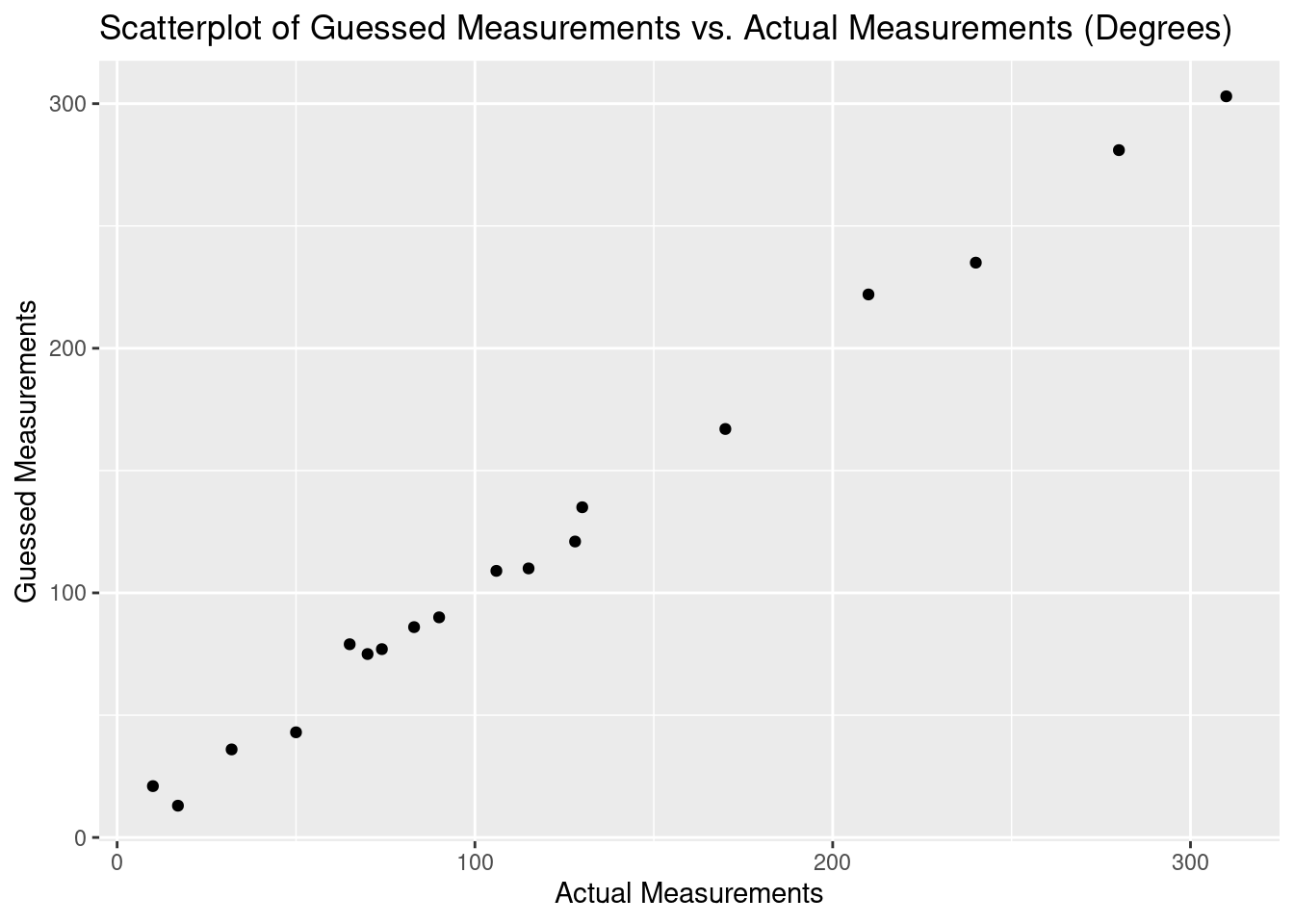
(2.1) Does the data appear to satisfy the criterion for a linear regression?

The data seems to be clearly exhibiting a linear relationship. Based on the scatterplot it seems appropriate to use a linear model here.

(2.2) Were the observations of the response variable collected independently? Is there any part of your data collection process that is intended to safeguard this assumption?

This is a difficult question to answer. It is possible that the estimations were not independent from one another. Though care was taken to ensure the correct measurements were hidden from the subject until the experiment was completely over, it is possible that previous estimations could have been used to inform future ones. This does not necessarily mean future estimations would be more accurate to the real measurement, as poor estimations informing future estimations would yield poor results, but the chance for true independence could have been hurt.

The author wonders if this is could be reasonably circumvented. Truly, even in psychometric evaluations one runs into the problem of previous answers potentially influencing future ones. Regardless, enough care was taken that the necessary assumptions are likely still valid.

(2.3) Residual Plots

residual_df <- data.frame(residual_list)
ggplot(residual_df, aes(x=residual_list)) +
    geom_histogram(bins = 18, color = "black") +
    theme_gray() +
    labs(x = "Residual Values", 
         y = "Frequency", 
         title = "Frequency Histogram of Residual Values")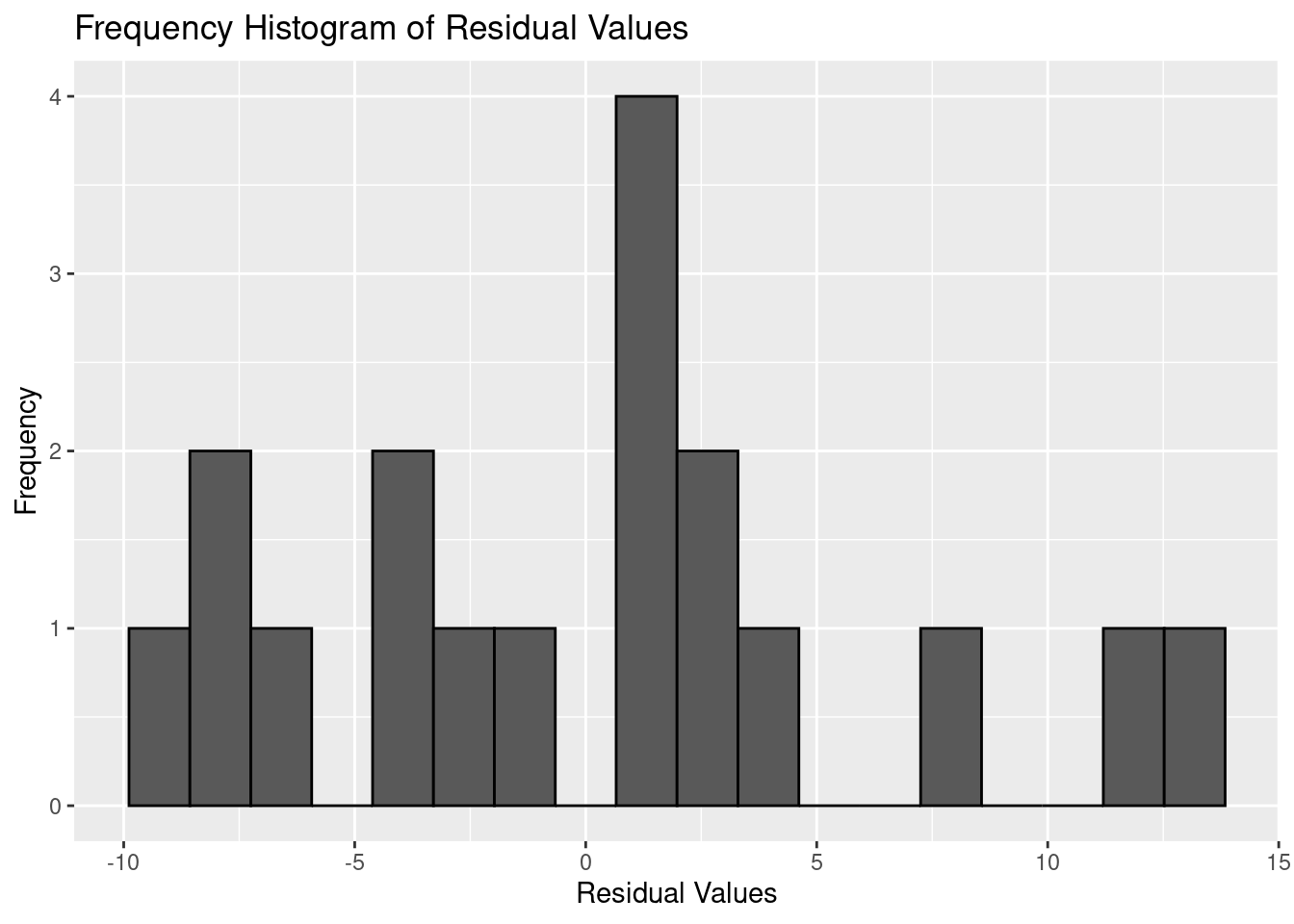

# Normal probability plot of the residual values
stand_df <- data.frame(y = rstandard(model))
ggplot(stand_df, aes(sample = y)) +
    stat_qq() + 
    stat_qq_line() +
    theme_gray() +
    labs(title = "Normal Probability Plot of Residual Values")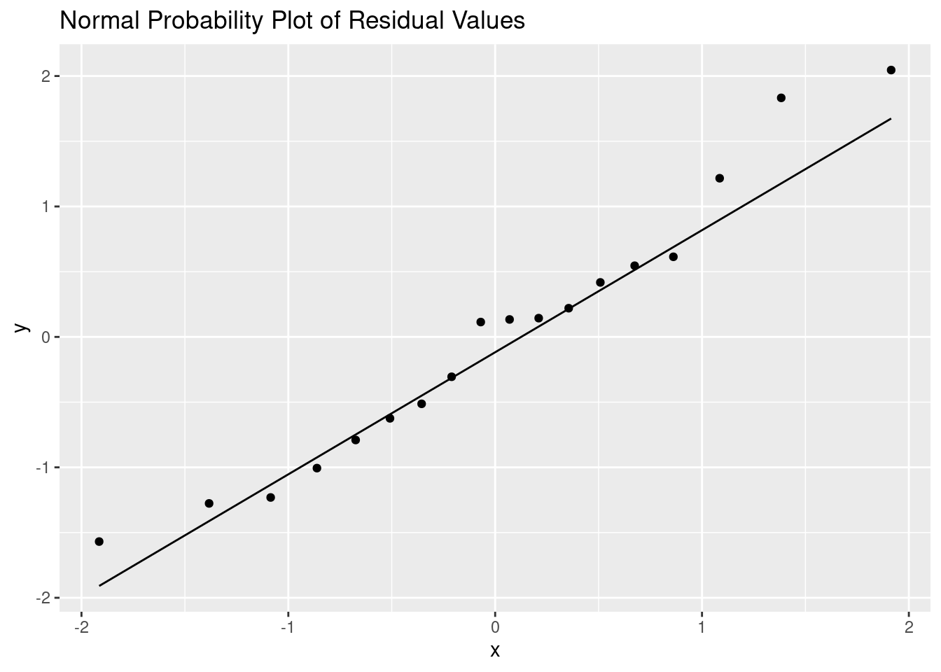

Based on the plots the normality assumption seems to be satisfied. The histogram appears relatively normal especially given a sample size of 18, and the normal probability plot of the residual values seems very linear as well.

(2.4) Residual Plots ctn. Constant Variance Assumption

ggplot(data = df, aes(x = actual, y = residuals(model))) +
  geom_point() +
  theme_gray() +
  stat_smooth(method = lm, se=FALSE) +
  labs(x = "Actual Measurement", 
       y = "Residual Values")

## `geom_smooth()` using formula 'y ~ x'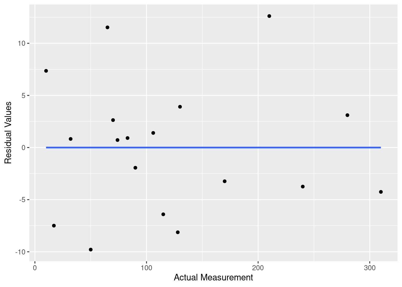

Based on the plot it does appear that constant variance assumption is satisfied. The amount of variance doesn’t really increase or decrease based on how big the actual measurement is. It is of note though, that none of the residuals after an actual angle measurement of 150 get quite as close as the small bundle of measurements around 80. Those measurements were very precise, but it is unclear if that precision is due to the size of the provided angle or not.

(3.1) Least Squares Regression Line

To calculate \(\hat{\beta_0}\) and \(\hat{\beta_1}\) we can pull up our model which thankfully has those values for us already.

model

## 
## Call:
## lm(formula = guess ~ actual, data = df)
## 
## Coefficients:
## (Intercept)       actual  
##      3.8565       0.9787

This gives us \(\hat{\beta_0} = 3.8565\) and \(\hat{\beta_1} = 0.9787\). Therefore, we get the following equation. \[f(x) = 3.8565 + 0.9787x\]

# scatterplot of the data WITH a regression line
ggplot(data = df, aes(x = actual, y = guess)) +
  geom_point() +
  theme_gray() +
  stat_smooth(method = lm, se=FALSE) +
  labs(x = "Actual Measurements",
       y = "Guessed Measurements",
       title = "Scatterplot of Guessed Measurements vs. Actual Measurements (Degrees)")

## `geom_smooth()` using formula 'y ~ x'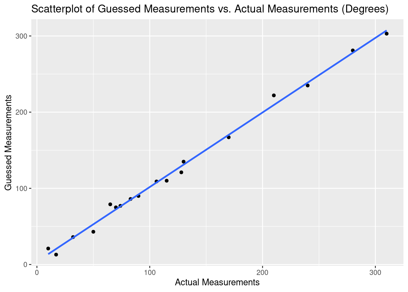

(3.2) Calculating a point estimate for the variance.

To calculate \(\hat{\sigma^2}\) we can utilize the following code. This value will also be, by construction, equal to \(\frac{SSE}{n-2}\).

sse <- sum((stats::predict(model) - df$guess)^2)
sigma_squared <- sse / (length(df$guess) - 2)

cat("The point estimate for sigma^2 is", round(sigma_squared,2))

## The point estimate for sigma^2 is 42.98

(3.3) Calculating \(r^2\)

To calculate \(r^2\) we can use the correlation function in R and square it. An alternative method to pull \(r^2\) directly from the models summary statistics without the rest of the summary’s clutter will also be used for the sake of comparison.

r_squared <- cor(df$actual, df$guess)^2
cat("R squared calculated using stats::cor() is",
    round(r_squared, 2))

## R squared calculated using stats::cor() is 0.99

cat("\nR squared as calculated by the model is",
    round(summary(model)$r.squared,2))

## 
## R squared as calculated by the model is 0.99

From this, it can stated that the proportion of variability in the actual measurements that is explained by the linear model relating estimated measurements to actual measurements is \(.99\). This value being so close to 1 means that almost all of the variability is explained by the linear model. This is as close to a perfect fit as one can reasonably expect to get.

(3.4) Constructing the Estimated Response Value

For this exercise we will let \(x^* = 270\). Plugging that value of x into our formula gives: \[f(270) = 3.8565 + 0.9787 \cdot 270 \approx \boxed{268.1}\]